Phase Matching for Nonlinear Optical Processes
This is a continuation from the previous tutorial - coupled-wave analysis of nonlinear optical interactions.
We have seen in the preceding tutorial the importance of phase matching for parametric nonlinear processes. If a parametric interaction is phase matched, optical power can be converted efficiently from one frequency to another. Otherwise, the process is periodically reversed, and the optical power shuttles back and forth among the interacting waves, as shown in Figure (9-8)(c) [refer to the coupled-wave analysis of nonlinear optical interactions tutorial]. No matter how long the crystal is, the best efficiency we can expect from a parametric interaction that is not perfectly phase matched is that contributed by the interaction over a coherence length. Therefore, phase matching is one of the most important technical issues that have to be addressed in designing any efficient nonlinear optical device based on a parametric frequency conversion process. In this tutorial, we discuss phase matching for second-order nonlinear optical processes.
The phase-matching condition of a nonlinear optical process is a relation among the wavevectors of the interacting waves. When more than two different wavevectors are involved, phase matching can be either collinear or noncollinear, as illustrated in Figure 9-9(a) and (b) for a second-order process. All of the wavevectors are parallel to each another in collinear phase matching, but they are not in noncollinear phase matching.

In the case of second-harmonic generation with only one input fundamental wave, phase matching is always collinear because there are only two wavevectors, \(\mathbf{k}_\omega\) and \(\mathbf{k}_{2\omega}\), involved in the process, as shown in Figure 9-9(c). However, noncollinear phase matching for second-harmonic generation is also possible if there are two spatially separated fundamental waves at the input, as shown in Figure 9-9(d). In the latter situation, the wavevectors of the two distinct fundamental waves can have different magnitudes if the two waves are not polarized in the same direction inside a birefringent crystal.
With noncollinear phase matching, the interaction length is limited by the finite distance over which the beams overlap in space. Therefore, the collinear phase-matching arrangement is employed in most nonlinear optical devices though noncollinear phase matching is also useful in some special applications. In the following, we consider only collinear phase matching for second-order nonlinear processes, but the general concepts can be easily extended to noncollinear phase matching. Phase matching for the third-order processes that are not automatically phase matched is difficult and rarely worth the effort because such processes are relatively inefficient.
With collinear beams, the phase-matching condition for a general second-order process reduces to the following simple scalar relation:
\[\tag{9-82}k_3=k_1+k_2,\qquad\text{or}\qquad{}n_3\omega_3=n_1\omega_1+n_2\omega_2\]
Efficient parametric interactions are normally carried out in a spectral region away from transition resonances of a medium to avoid attenuation of the optical beams due to resonant absorption of the medium. As discussed in the material dispersion tutorial and shown in Figure 22 [refer to the material dispersion tutorial], a material has normal dispersion in a spectral region away from resonances, meaning that \(n(\omega_3)\gt{n}(\omega_1),n(\omega_2)\). Clearly, collinear phase matching is not possible in an isotropic material or a cubic crystal within a spectral region of normal dispersion, nor is it possible in a birefringent crystal if all of the interacting waves have the same polarization. An isotropic material is of no practical use for second-order nonlinear interactions because \(\boldsymbol{\chi}^{(2)}=0\) in the electric-dipole approximation. A noncentrosymmetric cubic crystal, such as GaAs, has a decent \(\boldsymbol{\chi}^{(2)}\). However, such a crystal in bulk, homogeneous form is also not useful for second-order nonlinear optical interactions because of its inability to support collinear phase matching in the normal dispersion region where the crystal is transparent to the interacting optical waves. It is useful for second-order processes that are automatically phase matched, namely, the processes of optical rectification and Pockels effect.
Collinear phase matching can be achieved through the use of (1) anomalous dispersion near the resonance frequency of a material, (2) birefringence in a nonlinear crystal, (3) periodic spatial modulation in the nonlinear coefficient of a medium, or (4) modal dispersion of an optical waveguide. Among these possibilities, the use of anomalous dispersion is not very practical for device applications because of strong material absorption near a resonance frequency. The modal dispersion of a waveguide is usually not strong; thus it is also of limited usefulness.
Birefringent phase matching
The most commonly used method of obtaining collinear phase matching for a second-order nonlinear optical process employs the birefringence of a uniaxial or biaxial crystal. In the following, phase matching in uniaxial crystals is addressed specifically because it is less complicated than that in biaxial crystals. The same principles apply to phase matching in biaxial crystals.
As discussed in the propagation in an anisotropic medium tutorial, and illustrated in Figure 10 [refer to the propagation in an anisotropic medium tutorial], there are two normal mode polarizations, \(\hat{e}_\text{o}\) and \(\hat{e}_\text{e}\), associated with each direction \(\hat{k}\) of wave propagation in a uniaxial crystal. The ordinary wave with polarization \(\hat{e}_\text{o}\) has an ordinary refractive index \(n_\text{o}\) independent of the direction of \(\hat{k}\), whereas the extraordinary wave with polarization \(\hat{e}_\text{e}\) has an extraordinary refractive index \(n_\text{e}(\theta)\) that is given in (125) [refer to the propagation in an anisotropic medium tutorial] and is a function of the angle \(\theta\) between the \(\hat{k}\) vector and the optical axis. To satisfy the phase-matching condition in (9-82) in a spectral region of normal dispersion, the wave at the highest frequency, \(\omega_3\), has to be associated with the smaller of the two indices. Consequently, in a positive uniaxial crystal the wave at \(\omega_3\), or that at \(2\omega\) in the case of second-harmonic generation, has to be an ordinary wave, whereas in a negative uniaxial crystal it has to be an extraordinary wave.
There are two different types of birefringent phase-matching methods. In type I phase matching the two low-frequency waves have the same polarization, whereas in type II phase matching they have orthogonal polarizations. Note that in collinear phase matching, the \(\mathbf{k}\) vectors of the interacting waves are all parallel to one another. Therefore, their normal modes also have the same \(\hat{e}_\text{o}\) and \(\hat{e}_\text{e}\) vectors. Table 9-6 below summarizes the characteristics of type I and type II phase-matching methods for uniaxial crystals. In table 9-6, we have arbitrarily assigned for type II phase matching the wave at \(\omega_1\) to be the ordinary wave and that at \(\omega_2\) to be the extraordinary wave. When \(\omega_1\ne\omega_2\), there are two different possibilities of type II phase matching, with the ordinary wave at \(\omega_1\) being the one at either the lower or the higher frequency. The angle \(\theta_\text{PM}\) between vector \(\hat{k}\) and the optical axis that allows a particular phase-matching condition to be satisfied is known as the phase-matching angle.

In collinearly phase-matched second-harmonic generation, there is only one fundamental wave. In type I phase matching, the fundamental wave is completely polarized along one of the normal mode polarizations; thus the phase-matching condition is simply
\[\tag{9-83}n_{2\omega}=n_\omega\]
In type II phase matching, the fundamental wave consists of components in both normal mode polarizations. Therefore, the phase-matching condition becomes
\[\tag{9-84}n_{2\omega}^\text{o}=\frac{1}{2}\left[n_\omega^\text{o}+n_\omega^\text{e}(\theta_\text{PM})\right]\]
for a positive uniaxial crystal, or
\[\tag{9-85}n_{2\omega}^\text{e}(\theta_\text{PM})=\frac{1}{2}\left[n_\omega^\text{o}+n_\omega^\text{e}(\theta_\text{PM})\right]\]
for a negative uniaxial crystal. These different phase-matching methods for second-harmonic generation are illustrated in Figure 9-10 below.

We see from (122) [refer to the propagation in an anisotropic medium tutorial] that vector \(\hat{k}\) is a function of both \(\theta\) and \(\phi\). In a phase-matched interaction, the value of \(\theta\) is the phase-matching angle \(\theta_\text{PM}\), which is obtained by solving the condition for a specific phase-matching method. Phase matching in a uniaxial crystal is independent of angle \(\phi\). Therefore, the value of \(\theta_\text{PM}\) is determined without knowledge of \(\phi\). The value of \(\chi_\text{eff}\) is usually a function of both \(\theta\) and \(\phi\), however. For example, KDP is a negative uniaxial crystal of \(\bar{4}2m\) symmetry whose only nonvanishing second-order nonlinear susceptibility elements are \(\chi_{14}^{(2)}=\chi_{25}^{(2)}\) and \(\chi_{36}^{(2)}\) under the conditions for index contraction. Using (123) and (124) for \(\hat{e}_\text{o}\) and \(\hat{e}_\text{e}\), respectively, [refer to the propagation in an anisotropic medium tutorial], we find that \(\chi_\text{eff}=-\chi_{36}^{(2)}\sin\theta\sin{2\phi}\), or \(d_\text{eff}=-d_{36}\sin\theta\sin{2\phi}\), for type I phase matching and \(\chi_\text{eff}=\left(\chi_{14}^{(2)}+\chi_{36}^{(2)}\right)\sin\theta\cos\theta\cos{2\phi}\), or \(d_\text{eff}=(d_{14}+d_{36})\sin\theta\cos\theta\cos{2\phi}\), for type II phase matching. Therefore, to maximize the value of \(|\chi_\text{eff}|\) so that a second-order interaction in KDP is most efficient, \(\phi\) has to be chosen to have one of the values among \(\pi/4\), \(-\pi/4\), \(3\pi/4\), and \(-3\pi/4\) in the case of type I phase matching and one of the values among \(0\), \(\pi/2\), \(-\pi/2\), and \(\pi\) in the case of type II phase matching. In some crystals, notably uniaxial crystals of symmetry classes \(4\), \(6\), \(422\), \(622\), \(4mm\), and \(6mm\), \(\chi_\text{eff}\) is independent of angle \(\phi\) but is a function of \(\theta\) only. Then the value of \(\phi\) can be chosen arbitrarily, though that of \(\theta\) is still determined by the phase-matching condition.
For a specific nonlinear interaction in a given crystal, type I and type II phase matching methods generally have different phase-matching angles and different effective nonlinear susceptibilities. In certain cases, only one type of phase matching is possible. Sometimes, both types are not possible in a particular crystal within a certain spectral range. In case it is possible to have both type I and type II phase matching, the choice between the two depends on many practical considerations, including efficiency, angular tolerance, temperature sensitivity, and beam walk-off. Usually the one with the larger value of \(|\chi_\text{eff}|\) is chosen if it has no significant disadvantages from other considerations. Sometimes, \(\chi_\text{eff}\) vanishes when phase matching is achieved. Clearly, such phase matching is of no practical usefulness. A simple example is type II phase matching in KDP with \(\theta_\text{PM}=\pi/2\).
In summary, the condition for phase matching and the value of \(\chi_\text{eff}\) have to be considered at the same time when designing a practical device. Phase matching by itself does not guarantee a desirable value of \(\chi_\text{eff}\) and, in some special cases, can even lead to a vanishing \(\chi_\text{eff}\). For a collinearly phase-matched interaction in a uniaxial crystal, the value of \(\theta\) is determined by phase matching to be \(\theta=\theta_\text{PM}\), while that of \(\phi\) is determined by maximizing the value of \(|\chi_\text{eff}|\). In a biaxial crystal, the angle \(\theta\) is not independent of the angle \(\phi\), but they are determined by similar considerations. When both \(\theta\) and \(\phi\) are determined, the propagation direction \(\hat{k}\), which is common to all of the interacting waves in a collinear interaction, is fixed. In practice, a nonlinear crystal intended for a particular application is normally cut with the knowledge of the correct values of \(\theta\) and \(\phi\) for the application in a way that vector \(\hat{k}\) is normal to the input surface of the crystal and the \(\hat{e}_\text{o}\) and \(\hat{e}_\text{e}\) polarizations are along certain convenient directions in the experimental setup.
Example 9-8
Both type I and type II configurations of collinear birefringent phase matching are considered for second-harmonic generation in LiNbO3 with a fundamental wave at 1.10 μm. Find the polarization directions of the interacting waves, the phase-matching angle, and the nonlinear susceptibility for each type.
LiNbO3 is a negative uniaxial crystal of \(3m\) symmetry. The polarizations of the ordinary and extraordinary waves in a uniaxial crystal are \(\hat{e}_\text{o}=\hat{x}\sin\phi-\hat{y}\cos\phi\) and \(\hat{e}_\text{e}=-\hat{x}\cos\theta\cos\phi-\hat{y}\cos\theta\sin\phi+\hat{z}\sin\theta\), given in (123) and (124), respectively [refer to the propagation in an anisotropic medium tutorial]. According to Example 9-6 [refer to the coupled-wave analysis of nonlinear optical interactions tutorial], the nonvanishing nonlinear susceptibility tensor elements of LiNbO3 are \(d_{31}=d_{32}=d_{24}=d_{15}=-4.4\text{ pm V}^{-1}\), \(d_{22}=-d_{21}=-d_{16}=2.4\text{ pm V}^{-1}\), and \(d_{33}=-25.2\text{ pm V}^{-1}\). According to Example 9-7 [refer to the coupled-wave analysis of nonlinear optical interactions tutorial], the refractive indices of LiNbO3 are \(n_\text{o}=2.2319\) and \(n_\text{e}=2.1536\) at the fundamental wavelength of 1.10 μm and \(n_\text{o}=2.3168\) and \(n_\text{e}=2.2260\) at the second-harmonic wavelength of 550 nm. The extraordinary index at an angle \(\theta\) is given by (125) [refer to the propagation in an anisotropic medium tutorial] as \(n_\text{e}^{-2}(\theta)=n_\text{o}^{-2}\cos^2\theta+n_\text{e}^{-2}\sin^2\theta\).
For type I phase matching, we find from Table 9-6 that the fundamental is an ordinary wave with \(\hat{e}_\omega=\hat{e}_\text{o}\) and the second harmonic has to be an extraordinary wave with \(\hat{e}_{2\omega}=\hat{e}_\text{e}\). With the given nonvanishing nonlinear susceptibility elements, we find that the effective nonlinear susceptibility is
\[\tag{9-86}\chi_\text{eff}^\text{I}=\hat{e}_\text{e}\cdot\boldsymbol{\chi}^{(2)}:\hat{e}_\text{o}\hat{e}_\text{o}=\chi_{31}^{(2)}\sin\theta-\chi_{22}^{(2)}\cos\theta\sin3\phi\]
or, equivalently, \(d_\text{eff}^\text{I}=d_{31}\sin\theta-d_{22}\cos\theta\sin3\phi\). The phase-matching angle \(\theta_\text{PM}^\text{I}\) can be found by using the relation in (9-83) for \(n_{2\omega}^\text{e}(\theta_\text{PM}^\text{I})=n_\omega^\text{o}\). Using the formula for \(n_\text{e}(\theta)\), we find that
\[\tag{9-87}\theta_\text{PM}^\text{I}=\sin^{-1}\left[\frac{(n_\omega^\text{o})^{-2}-(n_{2\omega}^\text{o})^{-2}}{(n_{2\omega}^\text{e})^{-2}-(n_{2\omega}^\text{o})^{-2}}\right]^{1/2}=\sin^{-1}\left(\frac{2.2319^{-2}-2.3168^{-2}}{2.2260^{-2}-2.3168^{-2}}\right)^{1/2}=74.8^\circ\]
The angle \(\phi\) is chosen so that \(|d_\text{eff}^\text{I}|\) is maximized because \(\phi\) is irrelevant to phase matching in a uniaxial crystal. Because \(d_{31}\lt0\), \(d_{22}\gt0\), and \(0^\circ\le\theta\le90^\circ\), we can maximize \(|d_\text{eff}^\text{I}|\) by simply making \(\sin3\phi=1\) in (9-86). Therefore, \(\phi\) is chosen to be \(-90^\circ\), \(30^\circ\), or \(150^\circ\). We then find that \(d_\text{eff}^\text{I}=-4.88\text{ pm V}^{-1}\) and \(\chi_\text{eff}^\text{I}=-9.76\text{ pm V}^{-1}\) for \(\theta=74.8^\circ\) and \(\phi=-90^\circ\), \(30^\circ\), or \(150^\circ\).
For type II phase matching, we find from Table 9-6 that the fundamental is required to have both ordinary and extraordinary components but the second harmonic is an extraordinary wave with \(\hat{e}_{2\omega}=\hat{e}_\text{e}\). With the given nonvanishing nonlinear susceptibility elements, we find that the effective nonlinear susceptibility is
\[\tag{9-88}\chi_\text{eff}^\text{II}=\hat{e}_\text{e}\cdot\boldsymbol{\chi}^{(2)}:\hat{e}_\text{o}\hat{e}_\text{e}=\chi_{22}^{(2)}\cos^2\theta\cos3\phi\]
or, equivalently, \(d_\text{eff}^\text{II}=d_{22}\cos^2\theta\cos3\phi\).
The phase-matching angle \(\theta_\text{PM}^\text{II}\) can be found by using the relation in (9-85). Plugging the formula for \(n_\text{e}(\theta)\) into (9-85) results in a complicated algebraic relation, which can be either solved graphically or numerically to find that there is no solution for \(\theta_\text{PM}^\text{II}\) in the range from \(0^\circ\) to \(90^\circ\). Therefore, type II phase matching is not possible for second-harmonic generation in LiNbO3 at \(\lambda\) = 1.10 μm. The angle \(\phi\) can still be chosen so that \(|d_\text{eff}^\text{I}|\) is maximized because \(\phi\) is irrelevant to phase matching in a uniaxial crystal. In type II phase matching, \(|d_\text{eff}^\text{II}|\) can be maximized by making \(\cos3\phi=\pm1\) so that \(|\cos3\phi|=1\). For this purpose, \(\phi\) can be chosen as one of the following values: \(0^\circ\), \(\pm60^\circ\), \(\pm120^\circ\), or \(180^\circ\). Because phase matching is not possible, maximizing \(|d_\text{eff}^\text{II}|\) in this situation serves no practical purpose.
We can compare \(\chi_\text{eff}^\text{I}\) and \(\chi_\text{eff}^\text{II}\) obtained in (9-86) and (9-88), respectively, to see that for LiNbO3, type I interaction is more efficient than type II interaction.
Angle Tuning
The phase-matching angle for a specific interaction in a given nonlinear crystal is a function of the frequencies, or the wavelengths, of the interacting waves. When the frequencies of the interacting waves are varied, the angle \(\theta\) has to be varied accordingly for the interaction to remain phase matched. In practice, this angle tuning is normally carried out by rotating the crystal while maintaining the beam propagation direction though ti can also be achieved by varying the beam propagation direction while fixing the orientation of the crystal. One situation where this tuning is necessary is in an application with a wavelength-tunable input wave, such as in the generation of a wavelength-tunable difference- or sum-frequency wave or in the frequency doubling of the output from a wavelength-tunable laser. In optical parametric generation where only the pump-wave frequency at \(\omega_3\) is fixed, the parametrically generated frequencies \(\omega_1\) and \(\omega_2\) are varied when the parameters for phase matching are varied. Therefore, angle tuning of a nonlinear crystal is a convenient means for tuning the parametric wavelengths. Figure 9-11 below shows as an example the angle-tuning curves of the parametric wavelengths for type I and type II collinear phase matching in LiNbO3 with a fixed pump wavelength at 527 nm. LiNbO3 is a negative uniaxial crystal of \(3m\) symmetry, in which type I interaction is more efficient than type II interaction. The effective nonlinear susceptibilities for type I and type II phase matching in LiNbO3 are found in Example 9-8 and are given in (9-86) and (9-88), respectively.
 Figure 9-11. Angle-tuning curves showing parametric wavelengths as a function of the phase-matching angle for (a) type I and (b) type II collinear phase matching in LiNbO3 with a fixed pump wavelength at 527 nm. The data listed in Table 9-3 are used to generate these curves.
When the frequencies of the interacting waves are fixed, any deviation of the wave propagation direction away from the phase-matched direction results in a phase mismatch. The amount of this phase mismatch can be calculated by expanding \(\Delta{k}=k_1+k_2-k_3\) around the phase-matching angle:
\[\tag{9-89}\begin{align}\Delta{k}&=(k_1+k_2-k_3)_{\theta_\text{PM}}+\Delta\theta\left[\frac{\text{d}}{\text{d}\theta}(k_1+k_2-k_3)\right]_{\theta_\text{PM}}\\&\qquad+\frac{(\Delta\theta)^2}{2}\left[\frac{\text{d}^2}{\text{d}\theta^2}(k_1+k_2-k_3)\right]_{\theta_\text{PM}}+\ldots\\&=\frac{\Delta\theta}{c}\left(\omega_1\frac{\text{d}n_1}{\text{d}\theta}+\omega_2\frac{\text{d}n_2}{\text{d}\theta}-\omega_3\frac{\text{d}n_3}{\text{d}\theta}\right)_{\theta_\text{PM}}\\&\qquad+\frac{(\Delta\theta)^2}{2c}\left(\omega_1\frac{\text{d}^2n_1}{\text{d}\theta^2}+\omega_2\frac{\text{d}^2n_2}{\text{d}\theta^2}-\omega_3\frac{\text{d}^2n_3}{\text{d}\theta^2}\right)_{\theta_\text{PM}}+\ldots\end{align}\]
The acceptable angular tolerance in a nonlinear interaction is set by the amount of the acceptable phase mismatch. A common rule for setting this tolerance is \(\Delta{k}l\lt\pi\). In most applications of nonlinear optical devices, the interacting beams are focused to increase the efficiency. Because focusing increases the divergence, thus the angular spread, of a beam, an interaction that has a small angular tolerance requires the interacting beams to be well collimated and critically aligned.
Because \(n_\text{e}(0^\circ)=n_\text{o}\), a phase-matching angle in a uniaxial crystal cannot have the value of \(0^\circ\). Therefore, it can be shown by using (125) [refer to the propagation in an anisotropic medium tutorial] that \((\text{d}n_\text{e}(\theta)/\text{d}\theta)_{\theta_\text{PM}}\ne0\) except when \(\theta_\text{PM}=90^\circ\). If \(\theta_\text{PM}\ne90^\circ\), the first-order term in (9-89) exists; thus \(\Delta{k}\propto\Delta\theta\) approximately. For phase matching with \(\theta_\text{PM}=90^\circ\), known as \(90^\circ\) phase matching, the first-order term in (9-89) vanishes; thus \(\Delta{k}\propto(\Delta\theta)^2\). Because \(\Delta\theta\ll1\), \(90^\circ\) phase matching has a smaller phase mismatch for a given angular deviation or, equivalently, a larger angular tolerance for a given acceptable phase mismatch than phase matching with \(\theta_\text{PM}\ne90^\circ\). In \(90^\circ\) phase matching, an extraordinary wave is polarized along the optical axis, and \(n_\text{e}(90^\circ)=n_\text{e}\).
As can be seen from Table 9-6, for any method of birefringent phase matching, there is always at least one extraordinary wave involved in the interaction. For an extraordinary wave that is not polarized along a principal axis of a crystal, there is a walk-off angle \(\alpha\) given by (131) [refer to the propagation in an anisotropic medium tutorial] between its direction of propagation, defined by \(\hat{k}\), and its direction of power flow, defined by its Poynting vector \(\mathbf{S}\). In a collinear interaction, all of the interacting waves have the same direction of propagation, but not necessarily the same direction of power flow. When two interacting beams have different directions of power flow, there is a walk-off angle \(\rho\) between these two beams, which is defined as the angle between their Poynting vectors.

As shown in Figure 9-12(a), the walk-off angle between an ordinary beam and an extraordinary beam is simply \(\rho=|\alpha|\), which is determined only by the walk-off angle \(\alpha\) of the extraordinary beam. However, as illustrated in Figure 9-12(b), the walk-off angle between two collinear extraordinary beams is the difference of the walk-off angles of these two beams: \(\rho=|\alpha_1-\alpha_2|\), which exists between two extraordinary beams of different frequencies because of dispersion.
Because optical beams have finite transverse dimensions in reality, the existence of a walk-off angle \(\rho\) between two interacting beams limits the effective interaction length, as Figure 9-12 shows. For Gaussian beams with a radius \(w_0\) at the beam waist, the effective interaction length between two beams subject to the limitation of beam walk-off is the aperture distance:
\[\tag{9-90}l_\text{a}=\frac{\pi^{1/2}w_0}{\rho}\]
Clearly, the aperture distance decreases as the beams are increasingly focused.
When \(\theta=90^\circ\), an extraordinary wave is polarized along the extraordinary principal axis and thus has no walk-off, as can be verified with (131) [refer to the propagation in an anisotropic medium tutorial]. Consequently, there is no walk-off between any two interacting beams in the case of \(90^\circ\) phase matching. For this reason and for the reason discussed above that it has a larger angular tolerance than phase matching with \(\theta_\text{PM}\ne90^\circ\) has, \(90^\circ\) phase matching is called noncritical phase matching.
Example 9-9
A Gaussian beam of fundamental wave at 1.10 μm is used for second-harmonic generation with type I collinear angle phase matching in LiNbO3 discussed in Example 9-8. Find the walk-off angle \(\rho\) between the fundamental and second-harmonic beams. If the fundamental beam is focused to a waist size of \(w_0\) = 50 μm, what is the aperture distance limited by the walk-off effect?
For type I phase matching, only the second-harmonic beam, which is an extraordinary wave, has walk-off with an angle \(\alpha\) between \(\mathbf{S}_{2\omega}\) and \(\mathbf{k}_{2\omega}\). The fundamental beam is an ordinary wave with \(\mathbf{S}_\omega\parallel\mathbf{k}_\omega\). Therefore, the walk-off between the two Poynting vectors \(\mathbf{S}_\omega\) and \(\mathbf{S}_{2\omega}\), which is what matters in this interaction, is \(\rho=|\alpha|\) for collinear phase matching with \(\mathbf{k}_\omega\parallel\mathbf{k}_{2\omega}\). By using (131) [refer to the propagation in an anisotropic medium tutorial] for \(\alpha\) and taking the refractive indices to be \(n_\text{o}=2.3168\) and \(n_\text{e}=2.2260\) at the second-harmonic wavelength of 550 nm, we find, with \(\theta=\theta_\text{PM}=74.8^\circ\), the following walk-off angle:
\[\begin{align}\rho&=|\alpha|=\left|\tan^{-1}\left(\frac{n_\text{o}^2}{n_\text{e}^2}\tan\theta_\text{PM}^\text{I}\right)-\theta_\text{PM}^\text{I}\right|\\&=\left|\tan^{-1}\left(\frac{2.3168^2}{2.2260^2}\tan74.8^\circ\right)-74.8^\circ\right|=1.12^\circ=19.5\text{ mrad}\end{align}\]
For \(w_0\) = 50 μm, the aperture distance is
\[l_\text{a}=\frac{\pi^{1/2}w_0}{\rho}=\frac{\pi^{1/2}\times50\times10^{-6}}{19.5\times10^{-3}}\text{ m}=4.54\text{ mm}\]
The waist size of the second-harmonic beam is normally different from that of the fundamental beam. In the presence of walk-off, a second-harmonic beam generated by a circular Gaussian fundamental beam can have an elliptical spot shape. Such complications are ignored here.
Temperature tuning
It is clear from the above discussions that \(90^\circ\) phase matching is most desirable for both type I and type II phase-matching methods. In general, the ordinary and the extraordinary indices of a uniaxial crystal have different temperature dependencies, and the three principal indices of a biaxial crystal also change with temperature at different rates. In certain cases, it is possible to fix the angle \(\theta\) at \(90^\circ\) while varying the temperature to achieve phase matching. The temperature, \(T_\text{PM}\), at which \(90^\circ\) phase matching is achieved in a crystal is called the phase-matching temperature. Whether \(90^\circ\) phase matching by tuning the temperature is possible or not depends on the temperature dependence of the birefringence of a crystal, as well as on the wavelengths of the interacting waves in a given nonlinear process.
As discussed above, it is important to examine the value of \(\chi_\text{eff}\) at \(\theta=90^\circ\) for a given phase-matching method also. It turns out that \(\chi_\text{eff}=0\) for \(90^\circ\) phase matching in any uniaxial crystal if there are two extraordinary waves and one ordinary wave in the interaction, as well as in crystals of certain symmetry classes when there are two ordinary waves and one extraordinary wave in the interaction. Specifically, among all uniaxial crystals, \(90^\circ\) phase matching with \(\chi_\text{eff}\ne0\) is possible only for type I phase matching in a negative uniaxial crystal and for type II phase matching in a positive uniaxial crystal, but only if the crystal belongs to one of the symmetry classes \(3\), \(4\), \(6\), \(4mm\), \(6mm\), \(3m\), \(\bar4\), and \(\bar42m\) in either case. For biaxial crystals, the situation is more complicated.
Because the phase-matching temperature for a specific nonlinear interaction in a given crystal is a function of the frequencies of the interacting waves, it has to be tuned when the wavelengths of the waves are varied. Alternatively, in optical parametric generation with a fixed pump wavelength, the parametrically generated wavelengths can be tuned by tuning the temperature while keeping both the propagation direction of the beams and the orientation of the crystal fixed. Figure 9-13 shows as an example the temperature-tuning curves of the parametric wavelengths for type I and type II collinear phase matching in LiNbO3 with a fixed pump wavelength at 527 nm.

As shown in Figure 9-13 (b), temperature tuning with type II collinear phase matching for LiNbO3 is possible, but it is not practically useful because \(\chi_\text{eff}\) vanishes for type II \(90^\circ\) phase matching in LiNbO3. Therefore, temperature tuning for LiNbO3 is useful only with type I phase matching.
In temperature phase matching, deviation from the phase-matching temperature results in a phase mismatch given by
\[\tag{9-91}\begin{align}\Delta{k}&=(k_1+k_2-k_3)_{T_\text{PM}}+\Delta{T}\left[\frac{\text{d}}{\text{d}T}(k_1+k_2-k_3)\right]_{T_\text{PM}}+\ldots\\&=\frac{\Delta{T}}{c}\left(\omega_1\frac{\text{d}n_1}{\text{d}T}+\omega_2\frac{\text{d}n_2}{\text{d}T}-\omega_3\frac{\text{d}n_3}{\text{d}T}\right)_{T_\text{PM}}+\ldots\end{align}\]
For a practical device that is temperature tuned, the first-order term in (9-91) normally does not vanish. Therefore, \(\Delta{k}\propto\Delta{T}\) to first order.
In comparison with angle tuning, temperature tuning has all of the advantages of \(90^\circ\) phase matching discussed above. In addition, because the crystal orientation and the beam propagation direction are both fixed in a temperature-tuned device, temperature tuning also eliminates all of the troubles that come with angle tuning in mechanically changing the crystal orientation while trying to keep the optical beams aligned.
Example 9-10
In this example, we consider \(90^\circ\) phase matching in both type I and type II configurations for second-harmonic generation in LiNbO3 with a fundamental wave at 1.10 μm. The ordinary and extraordinary refractive indices of LiNbO3 as a function of wavelength and temperature are given by
\[\tag{9-92}n_\text{o}^2=4.9130+\frac{0.1173+1.65\times10^{-8}T^2}{\lambda^2-(0.212+2.7\times10^{-8}T^2)^2}-0.0278\lambda^2\]
\[\tag{9-93}\begin{align}n_\text{e}^2=4.5567&+2.605\times10^{-7}T^2\\&+\frac{0.0970+2.70\times10^{-8}T^2}{\lambda^2-(0.201+5.4\times10^{-8}T^2)^2}-0.0224\lambda^2\end{align}\]
where \(\lambda\) is the optical wavelength in micrometers and \(T\) is the temperature in kelvins. Use the data in Example 9-8 to find the polarization directions of the interacting waves, the phase-matching temperature, and the effective nonlinear susceptibility for each type.
For type I phase matching, the fundamental is an ordinary wave with \(\hat{e}_\omega=\hat{e}_\text{o}\), and the second harmonic has to be an extraordinary wave with \(\hat{e}_{2\omega}=\hat{e}_\text{e}\). The temperature, \(T_\text{PM}^\text{I}\), for \(90^\circ\) type I phase matching is found by solving \(n_{2\omega}^\text{e}(T_\text{PM}^\text{I})=n_\omega^\text{o}(T_\text{PM}^\text{I})\). Using the relations given in (9-92) and (9-93), we find the phase-matching temperature to be \(T_\text{PM}^\text{I}=396.7\text{ K}\), or \(123.7^\circ\). Because \(\theta_\text{PM}=90^\circ\) for \(90^\circ\) phase matching, we find from Example 9-8 that \(d_\text{eff}^\text{I}=d_{31}=-4.4\text{ pm V}^{-1}\) and \(\chi_\text{eff}^\text{I}=\chi_{31}^{(2)}=-8.8\text{ pm V}^{-1}\). Because \(\chi_\text{eff}^\text{I}\) does not depend on angle \(\phi\) in this situation, the value of \(\phi\) can be chosen arbitrarily.
For type II phase matching, the fundamental is required to have both ordinary and extraordinary components, and the second harmonic is an extraordinary wave with \(\hat{e}_{2\omega}=\hat{e}_\text{e}\). The temperature, \(T_\text{PM}^\text{II}\), for \(90^\circ\) type II phase matching is found by solving \(n_{2\omega}^\text{e}(T_\text{PM}^\text{II})=(n_\omega^\text{o}(T_\text{PM}^\text{II})+n_\omega^\text{e}(T_\text{PM}^\text{II}))/2\). Using the relations given in (9-92) and (9-93), we find that there is no solution for \(T_\text{PM}^\text{II}\). Therefore, \(90^\circ\) type II phase matching is not possible for second-harmonic generation in LiNbO3 at a fundamental wavelength of 1.10 μm. Combining this finding and that in Example 9-8, we find that type II phase matching is simply not possible for second-harmonic generation in LiNbO3 at 1.10 μm fundamental wavelength.
As demonstrated above in Figure 9-12, birefringent type II phase matching in LiNbO3 is possible for parametric generation at certain wavelengths. However, \(90^\circ\) type II phase matching in LiNbO3, and in any other crystal of \(3m\) symmetry alike, is useless anyway because \(\chi_\text{eff}^\text{II}=0\) for \(\theta=90^\circ\), as discussed in the discussions above and can be seen from (9-88).
For \(90^\circ\) collinear phase matching, there is no walk-off between \(\mathbf{S}_\omega\) and \(\mathbf{S}_{2\omega}\) because \(\mathbf{S}_\omega\parallel\mathbf{k}_\omega\parallel\mathbf{k}_{2\omega}\parallel\mathbf{S}_{2\omega}\). In this situation, the interaction is not limited by an aperture length because \(l_\text{a}=\infty\) effectively.
Quasi-phase matching
A very different phase-matching technique involves the introduction of a periodic modulation in a nonlinear medium. This approach is known as quasi-phase matching because phase mismatch is not eliminated within each modulation period but is compensated periodically. In principle, the periodic modulation can be on either the linear or the nonlinear susceptibility of the medium. In practice, however, modulating the linear susceptibility is less efficient than modulating the nonlinear susceptibility.
The principle of quasi-phase matching can be understood intuitively by following the discussions in the coupled-wave analysis of nonlinear optical interactions tutorial on the physical significance of the phase \(\varphi\) given in (9-67).
The existence of a phase mismatch \(\Delta{k}\) leads to a change of the phase \(\varphi\) by an amount of \(\pi\) over a coherence length, resulting in a change of sign in \(\sin\varphi\) and a reversal of the direction of energy flow in a parametric process. If the nonlinear susceptibility is periodically modulated such that a phase \(\varphi_\chi=\pi\) is introduced over each coherence length, the total phase \(\varphi\) is reset to its initial value so that the reversal of the process is prevented. Then energy can continue to flow in the desired direction.
The simplest and most effective approach to implementing such a periodic modulation is to change the sign of \(\boldsymbol{\chi}^{(2)}\) periodically, as illustrated in Figure 9-14(a) below. In ferroelectric nonlinear crystals, such as LiNbO3, LiTaO3, and KTP, the periodic sign change in \(\boldsymbol{\chi}^{(2)}\) can be achieved by periodic poling with an external electric field for periodic ferroelectric domain reversal. Periodically poled LiNbO3 (PPLN) and periodically poled KTP (PPKTP) are of great interest.
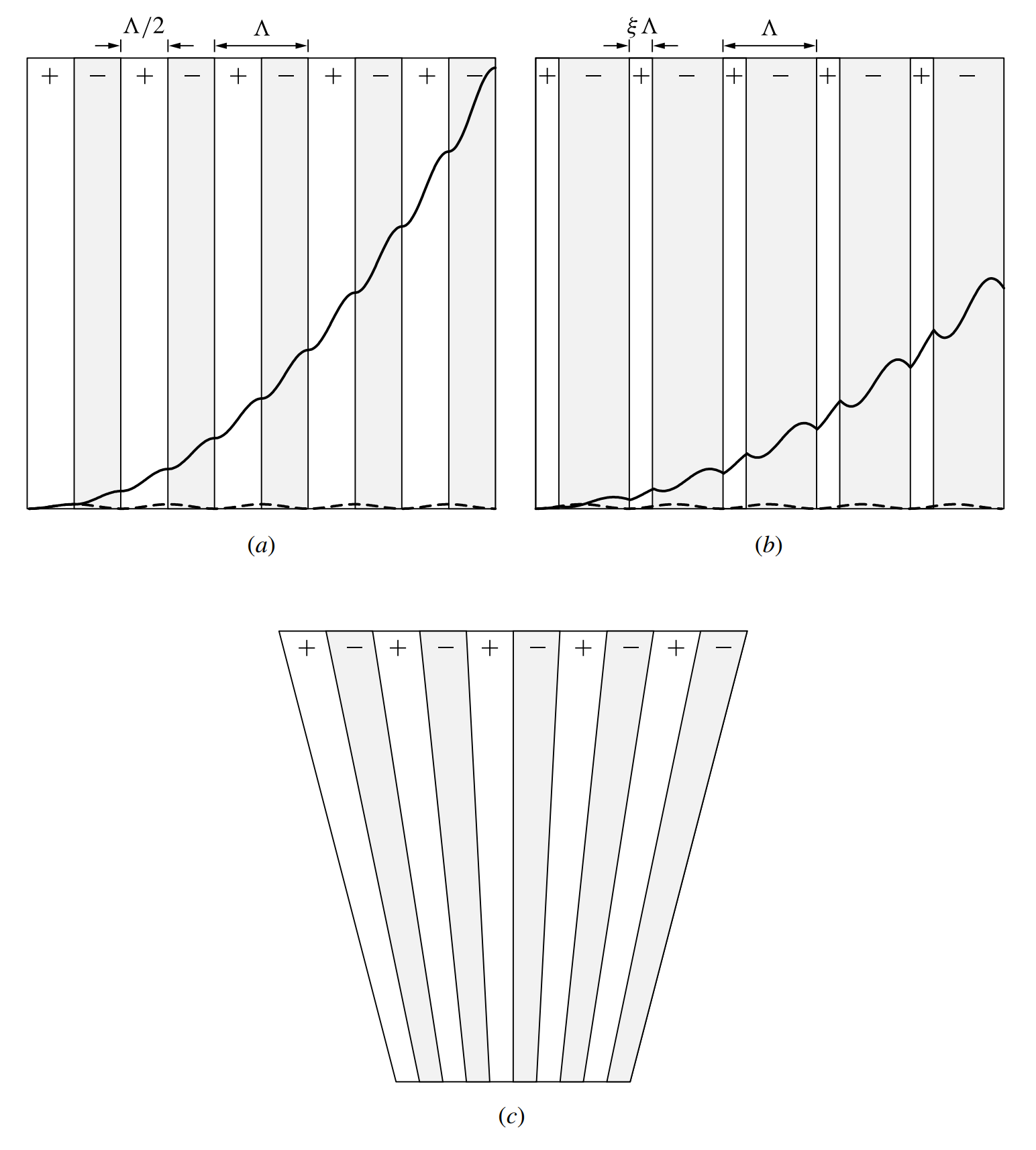
Any periodic modulation can be viewed as a grating. Therefore, the effect of a periodically modulated nonlinear susceptibility can be formally analyzed with a procedure similar to that used in the analysis of grating couplers in the grating waveguide couplers tutorial. In the presence of a periodic spatial modulation, the effective susceptibility defined in (9-59) [refer to the coupled-wave analysis of nonlinear optical interactions tutorial] becomes a periodic function of \(z\). It can be expressed in terms of a Fourier series expansion as
\[\tag{9-94}\chi_\text{eff}(z)=\sum_q\chi_\text{eff}(q)\text{e}^{\text{i}qKz}\]
where \(K=2\pi/\Lambda\), \(\Lambda\) is the modulation period, and
\[\tag{9-95}\chi_\text{eff}(q)=\frac{1}{\Lambda}\int_0^{\Lambda}\chi_\text{eff}(z)\text{e}^{-\text{i}qKz}\text{d}z\]
By substituting \(\chi_\text{eff}(z)\) of (9-94) for \(\chi_\text{eff}\) in (9-60) [refer to the coupled-wave analysis of nonlinear optical interactions tutorial], we have
\[\tag{9-96}\begin{align}\frac{\text{d}\mathcal{E}_3}{\text{d}z}&=\frac{\text{i}\omega_3^2}{c^2k_{3,z}}\mathcal{E}_1\mathcal{E}_2\sum_q\chi_\text{eff}(q)\text{e}^{\text{i}(\Delta{k}+qK)z}\\&\approx\frac{\text{i}\omega_3^2}{c^2k_{3,z}}\chi_\text{Q}\mathcal{E}_1\mathcal{E}_2\text{e}^{\text{i}\Delta{k}_\text{Q}z}\end{align}\]
where
\[\tag{9-97}\chi_\text{Q}=\chi_\text{eff}(q)\]
and
\[\tag{9-98}\Delta{k}_\text{Q}=\Delta{k}+qK\]
for an integer \(q\) that minimizes the value of \(|\Delta{k}+qK|\).
The other two coupled parametric equations in (9-61) and (9-62) [refer to the coupled-wave analysis of nonlinear optical interactions tutorial] can also be transformed in a similar manner. Therefore, all of the results obtained for parametric interactions discussed in the preceding section are still valid in the case of quasi-phase matching after making the substitution of \(\chi_\text{Q}\) and \(\Delta{k}_\text{Q}\) for \(\chi_\text{eff}\) and \(\Delta{k}\), respectively.
Perfect quasi-phase matching is achieved when \(\Delta{k}_\text{Q}=0\). This happens when the modulation period is chosen to be
\[\tag{9-99}\Lambda=-q\frac{2\pi}{\Delta{k}}=|q|\cdot2l_\text{coh}\]
Therefore, first-order quasi-phase matching occurs when \(\Lambda=2l_\text{coh}\) for \(q=1\) or \(-1\). Quasi-phase matching at a high order is also possible.
When designing a periodic structure for quasi-phase matching, it is important to maximize the value of \(\chi_\text{Q}\) to obtain the best efficiency for an interaction. In principle, any periodic structure is potentially useful. The simplest structure is one in which the sign of the nonlinear susceptibility is periodically reversed at abrupt boundaries. It is efficient and easy to fabricate. For such a structure with a duty factor \(\xi\), as shown in Figure 9-14(b) above, we find that
\[\tag{9-100}\begin{align}\chi_\text{Q}&=\frac{1}{\Lambda}\left[\int_0^{\xi\Lambda}\chi_\text{eff}\text{e}^{-\text{i}qKz}\text{d}z-\int_{\xi\Lambda}^\Lambda\chi_\text{eff}\text{e}^{-\text{i}qKz}\text{d}z\right]\\&=2\chi_\text{eff}\frac{\sin\xi{q}\pi}{q\pi}\text{e}^{-\text{i}\xi{q}\pi}\end{align}\]
which has a form similar to the coupling coefficient of a square grating found in (18) [refer to the grating waveguide couplers tutorial].
Note that the optimum value for the duty factor \(\xi\) depends on the order \(q\) of a structure. Clearly, a first-order structure with a 50% duty factor (\(\xi=1/2\)), which is shown in Figure 9-14(a) above, has the largest effective nonlinear susceptibility:
\[\tag{9-101}|\chi_\text{Q}|=\frac{2}{\pi}|\chi_\text{eff}|\]
For a given interaction, \(|\chi_\text{Q}|\) is always smaller than \(|\chi_\text{eff}|\).
It seems that an interaction with birefringent phase matching is always more effeicient than that with quasi-phase matching. This is not true, however.
In an interaction with birefringent phase matching, \(\chi_\text{eff}\) is subject to the constraints imposed by the phase-matching configuration on the propagation direction and the polarizations of the interacting waves. Therefore, other than choosing a proper angle \(\phi\) for the wave propagation direction and considering the difference between type I and type II phase-matching methods, there is little freedom in maximizing the effective nonlinear susceptibility when using birefringent phase matching.
Quasi-phase matching is not subject to such constraints because it depends on an externally imposed structure, rather than intrinsic material properties, for phase matching. Therefore, there is much freedom in seeking a high susceptibility in an interaction with quasi-phase matching.
For example, for LiNbO3, \(|\chi_{22}^{(2)}|\lt|\chi_{31}^{(2)}|\approx|\chi_{33}^{(2)}|/6\). From Examples 9-8 and 9-10, we find that \(|\chi_\text{eff}^\text{I}|\lt(|\chi_{31}^{(2)}|^2+|\chi_{22}^{(2)}|^2)^{1/2}\) and \(|\chi_\text{eff}^\text{II}|\lt|\chi_{31}^{(2)}|\) for type I and type II birefringent phase matching in LiNbO3, respectively. With birefringent phase matching, it is not possible to exploit the largest nonlinear susceptibility element \(\chi_{33}^{(2)}\) in LiNbO3 because \(\chi_{33}^{(2)}\) can be used only when all of the interacting waves are polarized along the extraordinary principal axis.
In contrast, with quasi-phase matching, all of the interacting waves can be polarized along the extraordinary axis so that \(\chi_\text{eff}=\chi_{33}^{(2)}\). If a first-order periodic modulation with a 50% duty factor is used for quasi-phase matching to compensate for the phase mismatch among the extraordinary waves, we have \(|\chi_\text{Q}|=2|\chi_\text{eff}|/\pi=2|\chi_{33}^{(2)}|/\pi\), which is about four times the value of \(|\chi_\text{eff}|\) for the most efficient interaction with type I or type II birefringent phase matching.
From the above discussions, it is clear that one important advantage of quasi-phase matching is that it makes possible efficient nonlinear interactions for which birefringent phase matching is not possible. Nonlinear interactions in nonbireringent nonlinear materials, such as III-V semiconductors, can also be phase matched with quasi-phase matching. The polarization directions of the interacting waves are not restricted in quasi-phase matching as they are in birefringent phase matching. This flexibility allows a collinear interaction within the transparency range of a nonlinear material to be noncritically phase matched with no beam walk-off at any temperature. High efficiency is possible by arranging the polarization directions of the waves for an interaction to use the largest susceptibility element of a nonlinear crystal. For wavelength tuning, the modulation period \(\Lambda\) has to be varied. With a fanned structure such as that shown in Figure 9-14(c) above, continuous wavelength tuning can be accomplished by translating the crystal transversely through the beam path.
Example 9-11
A PPLN crystal is used for second-harmonic generation of a fundamental beam at 1.10 μm wavelength. Find the required grating period for quasi-phase matching and the largest effective nonlinear susceptibility available for this interaction.
The largest susceptibility element of LiNbO3 is \(d_{33}=-25.2\text{ pm V}^{-1}\), thus \(\chi_{33}^{(2)}=2d_{33}=-50.4\text{ pm V}^{-1}\). From the above discussions, we know that both fundamental and second-harmonic waves have to be extraordinary waves polarized in the \(z\) direction in order to obtain the largest value of \(|\chi_\text{Q}|\) for a PPLN crystal. Therefore, we have to take \(n_\omega^\text{e}=2.1536\) for the fundamental wave at \(\lambda\) = 1.10 μm and \(n_{2\omega}^\text{e}=2.2260\) for the second harmonic at \(\lambda/2\) = 550 nm to calculate the phase mismatch \(\Delta{k}\) and the coherence length \(l_\text{coh}\) as in case (b) of Example 9-7 [refer to the coupled-wave analysis of nonlinear optical interactions tutorial]:
\[l_\text{coh}=\frac{\pi}{|\Delta{k}|}=\frac{\lambda}{4|n_\omega^\text{e}-n_{2\omega}^\text{e}|}=\frac{1.10\times10^{-6}}{4\times|2.1536-2.2260|}\text{ m}=3.80\text{ μm}\]
From the discussions following (9-100), we know that the largest value for \(|\chi_\text{Q}|\) is that given in (9-101) obtained with a first-order structure with a 50% duty factor. Therefore, the required grating period is
\[\Lambda=2l_\text{coh}=7.60\text{ μm}\]
For \(|q|=1\), and the effective nonlinear susceptibility is
\[|\chi_\text{Q}|=\frac{2}{\pi}|\chi_{33}^{(2)}|=32.08\text{ pm V}^{-1}\]
or, equivalently, \(|d_\text{Q}|=16.04\text{ pm V}^{-1}\).
In this scheme of quasi-phase matching, \(\mathbf{S}_\omega\parallel\mathbf{k}_\omega\parallel\mathbf{k}_{2\omega}\parallel\mathbf{S}_{2\omega}\) because both fundamental and second-harmonic fields are polarized along the principal \(z\) axis. Therefore, there is no walk-off between \(\mathbf{S}_\omega\) and \(\mathbf{S}_{2\omega}\). This interaction is not limited by an aperture length, which is effectively \(l_\text{a}=\infty\).
The next part continues with the optical frequency converters tutorial.