SPACE-DIVISION MULTIPLEXING AND MIMO PROCESSING

This is a continuation from the previous tutorial - Rate-adaptable optical transmission and elastic optical networks

 

 

1.  SPACE-DIVISION MULTIPLEXING IN OPTICAL FIBERS 

The capacity of fiber-optic communication systems has been increasing continuously by two to three orders of magnitude over the last two decades. Coherent optical communication has provided the most recent capacity improvements, reaching a performance close to the theoretical limit imposed on standard single-mode fibers \(\text{(SMFs)}\) by Shannon’s formula in combination with nonlinear effects.

In order to substantially increase the capacity of optical fibers, only one option, involving the introduction of multiple parallel optical paths, is left. The general technique is referred to a space-division multiplexing \(\text{(SDM)}\) and is the obvious choice for any interconnection technology if the capacity of a single serial channel reaches a technological barrier.

Space-division multiplexed system can be implemented by using multiple parallel \(\text{SMFs}\); in this form, however, no significant reduction of cost-per-bit can be expected and, therefore, around 2009 a new research effort in fiber optics communication started with the aim of identifying cost-efficient and scalable high-capacity \(\text{SDM}\) fiber systems

Two fiber types of particular interest emerged: The multicore fibers \(\text{(MCFs)}\), where multiple fiber guiding cores are introduced in a common cladding area and multimode fibers \(\text{(MMFs)}\), where the fiber modes are exploited to transmit multiple parallel channels. Both fiber types are well known but the design was now revisited and optimized for high-capacity transmission of parallel channels.

All \(\text{SDM}\) transmission systems can essentially be divided into two categories depending on the way the multiple parallel channels are processed at the receiver.

In uncoupled systems, each path is processed individually and any crosstalk from other channels will appear as impermanent limiting either the reach or the capacity of the individual channels.

The second approach is based on joint processing of the signals from the multiple parallel paths. The transmission system can then be described as a multiple-input multiple-output \(\text{(MIMO)}\) channel and well-known digital signal processing \(\text{(DSP)}\) techniques developed for wireless communication can be adopted.

In combination with coherent detection, it is then possible to practically undo any crosstalk between the channels as long as none of the channels is substantially attenuated in respect to the others.

The latter condition, which is typically not fulfilled in wireless systems, is often valid for low-loss optical components and multimode optical fibers.

In this tutorial consists of two main parts: \(\text{SDM}\) transmission and components. In the first part starting with OPTICAL FIBERS FOR SDM TRANSMISSION we describe various optical fibers that can support \(\text{SDM}\) transmission. 

In this OPTICAL TRANSMISSION IN SDM FIBERS WITH LOW CROSSTALK reviews \(\text{SDM}\) transmission techniques that can be utilized in case the crosstalk between the spatial channels is small, for example, in \(\text{MCFs}\).

IMPULSE RESPONSE IN SDM FIBERS WITH MODE COUPLING introduces the general principles for \(\text{SDM}\) transmission over optical fibers in the presence of coupling between the spatial channels, describes the basic properties of the fiber-optic multimode channel, such as differential group delay \(\text{(DGD)}\) and mode-dependent loss \(\text{(MDL)}\), and describes strategies to reduce the impact of the \(\text{DGD}\).

MIMO-BASED SDM TRANSMISSION RESULTS discusses experimental results for \(\text{MIMO}\) transmission and \(\text{MIMO}\) \(\text{DSP}\) techniques specific to SDM systems.

The second part of this tutorial describes methods for \(\text{SDM}\) component characterization and components required for \(\text{SDM}\) transmission systems such as mode couplers, \(\text{SDM}\) wavelength-selective switches \(\text{(WSSs)}\), and \(\text{SDM}\) optical amplifiers.

 

 

2.  OPTICAL FIBERS FOR SDM TRANSMISSION

In \(\text{SDM}\) transmission systems, multiple parallel optical paths are introduced to provide an increased link capacity. There are numerous ways to introduce multiple optical paths, and some representative approaches are graphically represented (drawn in scale) in Figure 1. for a spatial channel with a spatial multiplicity of 7. 

Figure 1(a) shows the state of the art approach consisting of conventional optical cable containing multiple standard \(\text{SMFs}\). Optical cables are widely available and can contain any number of fibers ranging from 1 to well over 1000. 

The second solution (see Figure 1(b)) consists of using fiber ribbons. This allows for an increase in fiber density of optical cables, and can reduce the time required to splice the optical cable, as fusion splicer for fiber ribbons are available and can splice a entire ribbon during a single splice operation.

A more recent approach that is not yet commercially available consists in the use of so-called multielement fibers, which are multiple fibers that after the draw are brought together and covered with a single common coating (see Figure 1(c)). Composite fibers can be packed much more densely together than individual \(\text{SMFs}\), and basically retain the same optical properties. The individual fibers are accessed by stripping the coating and are then handled similarly to regular \(\text{SMFs}\).

 

 

 

Further integration can be reached by using \(\text{MCFs}\), where multiple fiber cores share a common cladding and are, therefore, embedded physically in a single fiber (Figure 1(d)).

Splicing \(\text{MCFs}\) can be achieved by using a fusion splicer that is similar in functionality to fusion splicers designed for splicing polarization maintaining fibers, and therefore allows for splicing multiple spatial channels similarly as with ribbon splicer.

Connectors for \(\text{MCFs}\) have also been demonstrated  confirming that technologically \(\text{MCFs}\) are a viable solution for parallel interconnects. The placement of multiple core in a single cladding, however, also poses some new challenges.

To keep the crosstalk negligibly small, the cores have to be placed at a distance \(>40\mu m\) between each other, but the maximum practical cladding diameter is limited to \(250\;\mu m\) as the fiber becomes fragile and the bending radius tolerance becomes unpractical.

The realistic number of cores is currently limited to around 19, but new index profiles and various type of trances such as air holes, are currently under investigation to increase the maximum number of cores. 

The \(\text{MCF}\) design can be dramatically simplified if crosstalk between cores is allowed. The fibers are then referred to as coupled-core multicore fibers \(\text{(CC}\)-\(\text{MCFs)}\) or microstructured fibers (Figure 1(e)) and the cores can be placed much closer together.

The fiber will then behave similarly to a conventional \(\text{MMF}\), and the fiber modes are defined by the so-called “super-modes” that are the modes of the composite fiber refractive index profile including all cores. \(\text{CC}\)-\(\text{MCFs}\) currently under study have a core-to-core spacing from 22 to \(38\;\mu m\), but closer spaced cores have been proposed and analyzed in numerical studies.

In order to transmit parallel channels over \(\text{CC}\)-\(\text{MCFs}\) \(\text{MIMO}\) \(\text{DSP}\) techniques are required, and \(\text{CC}\)-\(\text{MCFs}\) will typically exhibit a strong mixing between the super-modes, which is advantageous to reduce the impact of core-to-core variation of the fiber optical properties. The implication of strong coupling on transmission is discussed in Multimode Fibers with Strong Mode Coupling.

Finally, the fibers that can achieve the highest density of spatial channels are \(\text{MMFs}\) (Figure 1(f)). \(\text{MMFs}\) have a core diameter or a core refractive index such as the resulting waveguide can support multiple spatial modes; this is in contrast to \(\text{SMFs}\) that only support a single spatial mode, however, with two polarizations.

The possibility to transmit multiple signals by making use of fiber modes has been proposed by Berdague and Facq. The concept was revitalized in 2000 by Stuart by proposing to apply \(\text{MIMO}\) \(\text{DSP}\) techniques to optical transmission over MMFs in order to increase either capacity or reach, followed by work form numerous other researchers.

Finally, in 2011, the idea was applied to the so-called few-mode fibers \(\text{(FMFs)}\) that are \(\text{MMFs}\) with only a small number of spatial modes (typically three or six spatial modes), and numerous long-distance and high-capacity demonstration have followed.

In contrast to the \(\text{MCF}\) approach where the challenge involves keeping the coupling between the core small, the challenge in \(\text{MMF}\) transmission is to minimize the transmission delay difference between the signals traveling over different modes.

This delay difference has to be minimized to contain the complexity of the \(\text{MIMO}\) \(\text{DSP}\) that is required to undo the coupling between modes and is addressed in detail in Digital Signal Processing for \(\text{MIMO}\) Transmission.

\(\text{MMFs}\) are not just advantageous because of their high spatial modal density, but offers several other significant advantages:

• Three to over 45 times the capacity of \(\text{SMFs}\) is possible while maintaining a standard cladding diameter of \(125\;\mu m\).
• \(\text{FMFs}\) are compatible with conventional fusion splices and also compatible with existing cabling and connector technologies.
• Most optical components such as splitters, isolators, circulators, wavelength combiners, and wavelength switches can be modified to support \(\text{MMFs}\) with a simple design modification.
• The strong-mode overlap in \(\text{FMFs}\) allows for efficient pump sharing in \(\text{FMF}\)-based optical amplifiers.

These are all important advantages that are partially offset, however, by the need of \(\text{MIMO}\) \(\text{DSP}\) to successfully recover the transmitted data. Note, however, that the complexity of \(\text{MIMO}\) \(\text{DSP}\) is addressable with current state-of-the-art \(\text{ASIC}\) technology. 

The list of approaches to implement \(\text{SDM}\) fibers shown in Figure 1 should give a good representative overview of the most promising technologies; additionally, it is noteworthy that many of the presented approaches can be combined.

Of particular interest are for example \(\text{MCFs}\) with few-mode cores as demonstrated, where up to 36 spatial channels have been demonstrated for a combination of uncoupled and \(\text{CC}\)-\(\text{MCFs}\).

 

 

3.  OPTICAL TRANSMISSION IN SDM FIBERS WITH LOW CROSSTALK

To overcome the capacity bottleneck represented by the \(\text{SMFs}\), multiple spatial paths have to be introduced. In order for the resulting \(\text{SDM}\) system to be cost effective in terms of cost of bit/s, further integration steps are essential. Integration can happen in any part of the optical transmission system, but will be most relevant in the part that contributes significantly to cost of the system, such as transceivers, reconfigurable optical add/drop multiplexers \(\text{(ROADMs)}\), optical amplifiers, and the optical fibers.

An often encountered side effect of integration is the increase of crosstalk between the spatial channels, which will typically grow significantly as function of the length of the transmission system. Managing the system crosstalk is, therefore, essential for SDM systems operated without digital crosstalk mitigation. In addition, the acceptable crosstalk level also depends on the format of the transmitted signal.

In Table 1, we report the maximum acceptable crosstalk level for a given added system penalty at a bit-error rate \(\text{(BER)}\) of \(10^{-3}\). Quadrature phase-shift keying \(\text{(QPSK)}\) is the most tolerant format and requires the crosstalk to be \(<−17\) dB for a added system penalty of 1 dB.

The requirements are more severe for higher-order modulation formats such as quadrature-amplitude modulation \(\text{(QAM)}\) format with 16 symbol \(\text{(16QAM)}\) where a minimum crosstalk of \(−23\) dB is required. 

The effect of accumulated crosstalk is particularly important in \(\text{MCFs}\), as the spatial channels share a common cladding. The theory describing coupling between parallel waveguides is referred in the literature as “coupled-mode theory” however, early experimental results clearly indicated that coupling in \(\text{MCFs}\) was not following the coupled-mode theory, which for the case of two cores predicts a sinusoidal transfer of the signals between cores as function of the distance.

The reason for the observed discrepancy is that multiple effects, such as fiber imperfection, and macro- and microbending, generally cause an almost random phase relation between the light propagating in different cores.

A new theory, the “coupled-power theory” was proposed by Fini et al.  and Hayashi et al. and applied to the design \(\text{MCFs}\) with minimum crosstalk also in practical bending scenarios.

Many different approaches to design \(\text{MCFs}\), such as the use of trenches, air holes, or even the use of cores with diverse phase velocity (referred to as heterogeneous cores), have been proposed by numerous groups and fibers with up to 19 cores have been successfully demonstrated. The main outcome from the coupled-power theory is that

TABLE 1.  Maximum acceptable crosstalk level for a given added system penalty observed at a bit-error rate of \(10^{-3}\) as a function of the modulation format

 

TABLE 2.  Summary of relevant \(\text{SDM}\) transmission in multicore fibers

 

the crosstalk accumulates linearly as function of the fiber length, which allowed the design of \(\text{MCFs}\) for long-distance transmission. Let us for example consider a system with 5000 km transmission based on \(\text{QPSK}\) signals.

The resulting crosstalk requirements for a single 100 km span is then a maximum crosstalk \(<−34\) dB, which can be easily achieved with seven core fibers. 

Numerous high-performance digital optical transmission experiments have been performed over \(\text{MCFs}\) by various groups. Some of the most significant results are summarized in Table 2. The maximum demonstrated capacity was over 1 Pbit/s in two cases, which are also the experiments with record high spectral efficiency, above 100 bit/s/Hz in one case.

In addition, there have also been significant long-distance results reaching distances up to 7326 km and record spectral-efficiency distance products above 200,000 bit/s/Hz km.

The \(\text{MCFs}\) research activities have been covering various aspects of \(\text{MCFs}\): New \(\text{OTDR}\) measurement techniques to characterize the \(\text{MCF}\) crosstalk, study of splices for \(\text{MCFs}\), connectors and even interoperability studies between \(\text{MCFs}\) from various fiber manufacturers, indicating that the technology is ready for real applications.

 

Digital Signal Processing Techniques for SDM Fibers with Low Crosstalk 

DSP techniques developed for \(\text{SMFs}\) can be directly applied to \(\text{MCFs}\) by treating every core independently and practically scale the capacity of the link up to the number of cores.

In \(\text{MCFs}\), it comes naturally to consider all signals in the individual cores as a single \(\text{SDM}\) channel, and the term “spatial super channel” has been coined to enforce the idea.

Spatial super channels offer significant advantages: for example, signals at a single wavelength can be transmitted over a spatial super channel by using a single wavelength. This can be used to significantly reduce the cost of the transceivers and to decrease the \(\text{DSP}\) complexity at the receiver.

In fact, all signals in the spatial channels that originate from a single laser will also exhibit similar phase noise, and it was proposed by Feuer et al. to use a single joint frequency offset compensation circuit for all spatial channels. Even proposed a device that can synchronize the phase noise between spatial channels.

The presence of multiple spatial channels can also be exploited to implement a self-homodyne transmission, where one spatial channel is used to transmit a copy of the unmodulated transmit laser as pilot tone to be used as local oscillator at the receiver.

The idea was originally proposed in \(\text{SMFs}\) where, for example, a polarization orthogonal to the signal can be used to transmit a pilot tone. The concept becomes more attractive in \(\text{MCFs}\) because by sacrificing a single core for the pilot tone transmission, only a modest reduction in the capacity has to be accepted. Self-homodyne transmission in \(\text{MCFs}\) has multiple benefits, and optimized phase recovery algorithms have been studied.

Self-homodyne detection makes the system much more insensitive to laser phase noise, allowing the use of low-cost distributed feedback laser \(\text{(DFB)}\) instead of the traditionally employed external cavity laser \(\text{(ECL)}\), which is a significant cost advantage.

Finally, the presence of multiple spatial modes can also be exploited to increase the sensitivity of the transmitted signal by sending multiple copies of the signal over different cores and digitally coherently superposing the multiple copies after receiving. The scheme was proposed and investigated in detail by Liu et al.

Furthermore, Liu et al. discovered that the sensitivity improvement could be further enhanced by sending multiple scramble copies of the signal. The received signals are then unscrambled and added coherently in the digital domain.

The scheme works because the scrambled signals will be impacted differently by the nonlinear fiber effects, and the reconstructed channels have less distortions than in the case where the signals are unscrambled and basically present highly correlated nonlinear distortions.

Using the technique, signal quality factor improvement of almost 5 dB by using three scrambled transmitted copies over a distance of 2688 km has been demonstrated. 

 

 

4.  MIMO-BASED OPTICAL TRANSMISSION IN SDM FIBERS

The main driver for \(\text{SDM}\) system cost reduction is integration of multiple spatial channels along all possible components of the transmission system. In many occasions, integration will also result in added crosstalk between the \(\text{SDM}\) channels. Crosstalk in low-loss fibers and optical components does not fundamentally degrade the information transmitted, but just mixes the transmitted signals.

For moderate transmission powers, the system can be approximated by a linear transmission function and the transmitted signals can then be recovered by applying the corresponding inverse linear transformation that undoes the mixing that occurs during transmission.

The principle is shown in Figure 2: Multiple signals \(s_1\cdots S_M\) are generated from a common laser and coupled into an \(\text{SDM}\) fiber by using an \(\text{SDM}\) multiplexer. The transmission system looks similar to a conventional single-mode system, except that all components such as fibers, optical amplifiers, or \(\text{WSSs}\) are

 

 

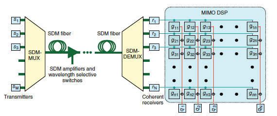
replaced with their \(\text{SDM}\) counterparts. At the receiver, an \(\text{SDM}\) demultiplexer separates the signals by spatial channels, and the signals \(r_1\cdots r_N\) are received by coherent receivers and fed into the \(\text{MIMO}\) \(\text{DSP}\) block that is capable of undoing all linear impairments of the transmission system and giving the reconstructed signals \(q_1\cdots q_N\) as output.

The \(\text{MIMO}\) \(\text{DSP}\) found in \(\text{SDM}\) systems can be considered an extension of the \(2\times2\) \(\text{MIMO}\) \(\text{DSP}\) encountered in polarization multiplexed system as described, for example, in this tutorial POLARIZATION AND NONLINEAR IMPAIRMENTS IN FIBER COMMUNICATION SYSTEMS, and is addressed in more detail in Digital Signal Processing for MIMO Transmission.

If nonlinear effects are neglected, the \(\text{SDM}\) transmission system can be described by the linear \(N\times M\) channel matrix \(h_{j,k}\), where each element of the matrix contains the complex amplitude impulse response for a particular pair of \(M\) input signals and \(N\) output signals.

\[\tag{1}r_j(l)=\boldsymbol{\sum}^{L_h}_{m=1}h_{j,k}(m)\cdot S_k(l+m-m_o)\]

where \(s_k(l)\) is the signal transmitted on channel \(k\) at discrete time index \(l\), \(r_j(l)\) is the signal received on channel \(j\) at discrete time index \(l\), and \(m_o\) is a constant that accounts for the overall propagation delay occurring in the \(\text{MIMO}\) channel.

For practical purposes, it is convenient to rewrite Equation 1. in a form that can be evaluated using conventional matrix multiplication rules.We define the matrix \(H\) describing the \(\text{SDM}\) system and the vectors \(s(l)\) and \(r(l)\) describing the input and output signals, respectively, as 

 

\[\tag{3}s(l)=\left[\begin{align}s_1(l-&m_0+1)\\s_1(l-&m_0+2)\\&\vdots\\s_1(l-&m_0+L_h)\\s_2(l-&m_0+1)\\s_2(l-&m_0+2)\\&\vdots\\s_M(l-&m_0+1)\\s_M(l-&m_0+2)\\&\vdots\\s_M(l-&m_0+L_h)\end{align}\right],\;\text{and}\] 

\[\tag{4}r(l)=\left[\begin{align}r_1&(l)\\r_2&(l)\\&\vdots\\r_N&(l)\end{align}\right]\] 

and Equation 1. can then be rewritten in matrix form as

\[\tag{5}r(l)=\boldsymbol{H}\cdot s(l)\]

Equation 5 calculates the output vector \(\boldsymbol{r}(l)\) for only one particular time index \(l\), and in practice it is desirable to expand the equation to include values for multiple time indices.

This can be achieved by expanding the vectors \(\boldsymbol{s}(l)\) and \(\boldsymbol{r}(l)\) into the corresponding matrices \(\boldsymbol{S}(l)\) and \(\boldsymbol{R}(l)\) defined as

 

Finally, the \(\text{SDM}\) system can be described as multiplication between two matrices in the following simple form:

\[\tag{7}\boldsymbol{R}=\boldsymbol{H}\cdot\boldsymbol{S}\]

In a practical \(\text{SDM}\) transmission experiment, the transmitted signal \(\boldsymbol{S}(l)\) is formed by the chosen test pattern, for example, a De Bruijn bit sequence \(\text{(DBBS)}\), and the received signal \(\boldsymbol{R}(l)\) captured by a multichannel real-time digital oscilloscope, and the system channel matrix \(\boldsymbol{H}\) can then be estimated by multiplying Equation 8 from the right side with the pseudoinverse of the matrix \(\boldsymbol{S}\). We obtain

\[\tag{9}\hat{\boldsymbol{H}}=\boldsymbol{R}\cdot\boldsymbol S^*\cdot(\boldsymbol{S}\cdot\boldsymbol{S}^*)^{-1}\]

where \(*\) denotes the conjugate transpose operation and \(\hat{H}\) is the \(\text{SDM}\) channel estimation according to the least square criterion. 

The estimated matrix \(\hat{H}\) contains all combination of input–output impulse responses and is an important tool to study the transmission performance limitations in \(\text{SDM}\) systems.

It contains information such as the maximum delay spread and the maximum capacity estimate, and it can also be used to analyze the temporal evolution of the \(\text{SDM}\) system. 

In addition, the channel matrix can be further analyzed by performing a singular value decomposition \(\text{(SVD)}\), where the channel matrix is decomposed according to

\[\tag{10}\hat{H}=\boldsymbol{U}\cdot\boldsymbol{\Lambda V}^*\]

where \(\boldsymbol{U}\) and \(\boldsymbol{V}\) are unitary matrices and the rectangular diagonal matrix \(\boldsymbol{\Lambda}\) contains the real and positive singular values \(\lambda_1\cdots\lambda_N\).

The singular values squared \(\lambda^2_i\) represent the intensity transfer functions for the spatial paths transmitted through the \(\text{SDM}\) system. The ratio between the smallest and the largest singular values squared is defined as \(\text{MDL}\) according to

\[\tag{11}\text{MDL}_{\text{A}\Lambda G}=10*\text{log10}\left(\frac{\text{max}(\lambda^2_i)}{\text{min}(\lambda^2_i)}\right)\]

and is an important indicator for the system performance that can be expected for the \(\text{SDM}\) channel.

The linear \(\text{MIMO}\) channel matrix as defined in Equation 1 implicitly includes a convolution between the input signal and the output signal pairs. When transforming the channel matrix from the time domain into the frequency domain, the convolution will be replaced with a simple multiplication and the \(\text{SDM}\) system can then be described as

\[\tag{12}\boldsymbol{\tilde{r}}(\omega)=\boldsymbol{\hat{H}}(\omega)\cdot\boldsymbol{\tilde{s}}(\omega)\]

where the transmitted signal vectors \(\boldsymbol{\tilde{s}}(\omega)\) has \(M\) elements and the received signal vector \(\boldsymbol{\tilde{r}}(\omega)\) has \(N\) elements corresponding to the input and output channels, respectively. The frequency channel matrix is related to the time-domain channel matrix by the Fourier transform along the time index m of \(h_{j,k}(m)\) for each combination of input and output channels \(j\), \(k\).

The channel matrix represented in the frequency domain also offers the advantage that the total channel matrix of multiple cascaded \(\text{SDM}\) subsystems can be obtained by the matrix multiplication of the subsequent subsystem matrices. 

The concept of \(\text{MDL}\) is often also applied to the channel matrix in the frequency domain. The singular values are then evaluated for each individual frequency components and the resulting \(\text{MDL}\) becomes frequency dependent

\[\tag{13}\text{MDL}(\omega)=10*\text{log10}\left(\frac{\text{max}(\tilde{\lambda}^2_i(\omega))}{\text{min}\tilde{(\lambda}^2_i)(\omega)}\right)\]

which is particularly relevant for characterization of components as described in Characterization of \(\text{SDM}\) Systems and Components. The \(\text{MDL}\) of the channel matrix can exhibit strong frequency dependence, and fading dips are often observed in long-distance \(\text{MIMO}\) transmission experiments that can dramatically impact the performance of orthogonal frequency-division multiplexed \(\text{(OFDM)}\) \(\text{MIMO}\) system. 

 

 

5. IMPULSE RESPONSE IN SDM FIBERS WITH MODE COUPLING

In order to better understand mode coupling in a \(\text{SDM}\)9 fiber, it is instructive to study the spatial modes supported by the fiber. Modes in optical fibers are solutions of the Maxwell equation in a dielectric material that are invariant along the propagation direction.

The solutions of the mode equation can be calculated analytically for a few special cases, such as for fibers with a step-index profile where the solutions are Bessel functions, or for graded-index fibers where the solutions are Laguerre–Gaussian functions.

The latter are reported as examples in Figure 3. In general, the modes can be calculated numerically using mode solvers that are based on finite-element methods. The solution of the mode equation provides not only the spatial amplitude and phase, but also the propagation constant \(\beta _n\) of the corresponding mode \(n\).

The propagation constant is wavelength dependent and depends both on the material dispersion and the refractive index profile of the waveguide.

In general, the propagation constant can be approximated by the Taylor expansion 

\[\tag{14}\beta_n(\omega)=\beta_{0,n}+\beta_{1,n}(\omega-\omega_0)+\frac{1}{2}\beta_{2,n}(\omega-\omega_0)^2+\frac{1}{6}\beta_{3,n}(\omega-\omega_0)^3,\]

where \(\omega\) is the angular frequency of the light. The phase velocity that describes the speed at which a constant phase front travels along the waveguide is given by

\[\tag{15}v_{ph,n}=\frac{\omega_0}{\beta_{0,n}}.\] 

The second term of Equation 14 is related to the group velocity, which describes the propagation speed of light pulses in the fiber and is defined as

\[\tag{16}v_{gr,n}=\frac{1}{\beta_{1,n}}.\]

 

 

Finally, the third term of Equation 14.  is related to the chromatic dispersion coefficient, which is defined as 

\[\tag{17}cd_n=\frac{2\pi c}{\lambda^2}\beta_{2,n},\]

where \(c\) is the speed of light in vacuum, and \(\lambda=2\pi c/\omega\) is the wavelength of the light.

Modes are independent solutions of the mode equation and are orthogonal to each other, and form a full orthogonal set describing all the possible waves that can propagate through the waveguide.

Perfect waveguides do not show couplings between the modes; however, in real fibers, small variations in refractive index, and fiber geometry or bends in the fibers can cause modes to couple.

The relative phase velocity between two modes is an important parameter in determining the coupling between the modes. Modes that have almost the same phase velocity and also degenerate modes that have exactly the same phase velocity can be easily coupled by small perturbation, whereas generally less coupling is observed between modes with larger difference in phase velocity.

Alternatively, the effect of the difference in phase velocity can be transformed into the so-called beat length \(L_{n,m}\) defined as

\[\tag{18}L_{n,m}=\frac{2\pi}{|\beta_{0,n}-\beta_{0,m}|}\]

which is indicative of the length scale over which the coupling occurs. Because mode coupling is caused by multiple distributed fiber imperfections, it is difficult to identify the exact cause of the coupling. Numerous models have been proposed to describe mode coupling in \(\text{SDM}\) fibers under various assumptions such as slight offset of the cores in different fiber sections or the introduction of a generalized Stokes space and relative coupling matrix.

The group velocity difference is also a very important parameter, as it determines the maximum time delay between the received signals and, therefore, directly determines the number of equalizer taps necessary to completely undo the effect of mode coupling. The \(\text{DGD}\) between two modes of a fiber can be calculated by 

\[\tag{19}\text{DGD}_{n,m}=L_F|\beta_{1,n}-\beta_{1,m}|\]

where \(L_F\) is the fiber length. \(\text{MMF}\) designs that minimize the \(\text{DGD}\) across a wide wavelength range are, therefore, essential. The conventional step-index fiber modified to support multiple mode has typically more than 1 ns/km of \(\text{DGD}\), which makes \(\text{MIMO}\) transmission impractical to more than 50 km.

Various fiber designs to minimize the \(\text{DGD}\) of \(\text{MMFs}\) have been proposed; the most common are depressed cladding \(\text{(DC)}\)-based designs, ring-core fibers \(\text{(RC)}\), and graded-index \(\text{(GI)}\) profile fibers.

\(\text{MMFs}\) with graded-index profiles are also popular in short-distance interconnects and can theoretically have very small \(\text{DGD}\) values. They also offer other interesting properties, such as having a very similar difference in phase velocity between subsequent mode groups, and therefore optimally utilize the index contrast provided by the doping profile.

The first eight mode groups of a graded-index fiber are shown in Figure 3. Each subsequent mode group contains one additional spatial mode, and all modes within a mode group are nominally degenerate. Graded-index MMFs are the most often used fibers in \(\text{MIMO}\)-based SDM experimental demonstrations.

Optimized MMFs have typical \(\text{DGD}\) values around 30–100 ps/km for fiber with six or less spatial modes. Consistent fabrication of MMFs with smaller \(\text{DGD}\) values is difficult as the relative group velocity error has to be controlled to an accuracy of better than 1 ppm. 

In practice, when measuring the total intensity impulse response of an \(\text{MMF}\), three different scenarios, represented graphically in Figure 4 for an hypothetical MMF with two spatial modes, can occur. Note that all three scenarios can be encountered in

 

 

 

the same \(\text{MMF}\) just by varying the transmission length, which is graphically indicated by an arrow in Figure 4. All three scenarios have been experimentally investigated and are discussed later in detail. 

 

Multimode Fibers without Mode Coupling 

In the first scenario, mode coupling is negligible, and the impulse response consists of two delayed peaks separated by \(\text{DGD}\) between the two modes. This situation can be observed in short sections of MMFs. It is then possible to transmit independent signals over each mode without the need of \(\text{MIMO}\) \(\text{DSP}\). Early \(\text{SDM}\) demonstrations used this scheme to transmit over distances up to 10 km using direct modulation and detection.

A more advanced scheme employing \(\text{LP}_{01}\) and \(\text{LP}_{11}\) modes used 2 × 2 MIMODSP to transmit over the LP01 mode and \(4\times4\) \(\text{MIMO}\) \(\text{DSP}\) to transmit over the degenerate \(\text{LP}_{11}\) modes of an \(\text{MMF}\) with three spatial modes, reaching a transmission distance of up to 40 km based on a \(\text{QPSK}\) transmission signal.

The scheme was also applied to a fiber with five spatial modes reaching a distance of 40 km.

The scheme requires mode couplers with high modal selectivity, but ultimately the crosstalk build-up in the fibers themselves are limiting the transmission distance to \(<100\text{km}\). 

 

Multimode Fibers withWeak Coupling

In the second scenario, a weak crosstalk is present and produces an almost random uniform crosstalk plateau between the peaks corresponding to the undisturbed modes. The crosstalk plateau is generated by the light coupling between modes, which happens all along the fiber propagation, and a particular time position on the plateau can then be mapped to a location in the fiber where the coupling occurs.

For homogeneous fibers, the plateau will have a constant envelop, and defects, such as splices present in the fiber span, will generate localized peaks. In this scenario, the accumulated crosstalk of the whole plateau is large enough to require \(\text{MIMO}\) \(\text{DSP}\) to compensate for it, and the distance between the peaks is still determined by the \(\text{DGD}\) between the 

fiber modes and, therefore, will determine the minimum depth of the \(\text{MIMO}\) equalizer memory. For long-distance communication (1000 km or more), the \(\text{DGD}\) of an optimized MMF is still too large, and additional strategies are required to mitigate the effects of \(\text{DGD}\).

The strategy involves cascading the MMF with a second optical element that has the inverse \(\text{DGD}\) effect: The compensating element can be an \(\text{MMF}\) with corresponding negative \(\text{DGD}\) values or a \(\text{DGD}\) compensator according to Figure 18.

The \(\text{DGD}\) compensation is presented graphically in Figure 5, where the group delay as function of the distance is shown in a \(\text{DGD}\)-compensated fiber span, showing the modes separating in time during the first section of fiber and then overlapping at the end of the fiber span after traversing a section of the fiber with the inverse \(\text{DGD}\). 

Understanding the benefits of \(\text{DGD}\) compensation in the presence of modal crosstalk is somewhat counterintuitive. In fact, the mode coupling between non-degenerate modes, which can be as large as 8% for a 100 km \(\text{GI}\)-\(\text{MMF}\) span, can happen at any location along the compensated span and, therefore, produce copies of the signal delayed by amounts up to the \(\text{DGD}\) of the uncompensated fiber.

The inherent advantage of \(\text{DGD}\) compensation, which is to limit the spread of the system impulse response, is therefore not apparent anymore.

Nevertheless, the following simulations and experimental results confirm \(\text{DGD}\) compensation to be effective, but only in multispan systems, and under the condition that the majority of the optical power stays in the mode it was launched into.

If the last condition is not fulfilled, strong coupling will reduce the impact of \(\text{DGD}\) as described in Multimode Fibers with Strong Mode Coupling \(\text{DGD}\) compensation can be performed at a span level or also within a span. Deployed fibers typically consist of multiple cables that are spliced every kilometer, and it is, therefore, conceivable to perform \(\text{DGD}\) compensation by splicing cables with \(\text{DGD}\) values with alternating sign.

The effect of \(\text{DGD}\) compensation is demonstrated in Figure 6, where the sum of all intensity responses is simulated for link lengths

 

 

 

 

of 100, 200, 500, 1000, 2000, and 5000 km, based on a 100-km spans, and reported for (a) \(\text{DGD}\) uncompensated spans, (b) \(\text{DGD}\) compensated spans, and (c) spans compensated every kilometer.

The simulations are based on a simple model, which uses incoherent convolutions to determine the effects of cascaded spans and additionally mode couplers with strong coupling are assumed after each span.

Other simulation parameters are as follows: 8% distributed mode coupling between non-degenerate modes per span, 1% mode coupling at splice locations, fibers with 50 ps/km \(\text{DGD}\), and a residual not compensated \(\text{DGD}\) of 100 ps after each span.

The results demonstrate the efficacy of \(\text{DGD}\) compensation, as can be observed by comparing the different time scale for (a), (b), and (c) in Figure 6. When \(\text{DGD}\) compensation is applied at every span, the spread of the impulse response is reduced by a factor of 5. Furthermore, when \(\text{DGD}\) compensation is performed every kilometer, the impulse response spread is reduced by an additional factor of 50. \(\text{DGD}\) compensation was also confirmed experimentally, performing recirculating loop experiments in \(\text{FMF}\) with three and six spatial modes.

The total intensity responses are reported for different propagation distances in Figure 7(a) and (b), for 30-km FMF with three spatial modes and 59-km FMF with six spatial modes, respectively. Both fibers were \(\text{DGD}\) compensated and show a strong central peak after traversing the fiber the first time.

In the subsequent loop traversals, the width of the impulse response stays contained within the \(\text{DGD}\) compensation windows as long as the central peak is dominating. At longer distances, the impulse response changes to a bell-shaped curve and will transit into the strong coupling regime as described in Section Multimode Fibers with Strong Mode Coupling

 

 

 

Multimode Fibers with Strong Mode Coupling 

The third scenario that can be encountered in \(\text{MMFs}\) is the so-called strong coupling regime, where the coupling between the modes is so strong to continuously mix the signals between the modes. The strong coupling regime is beneficial for reducing the effect of \(\text{DGD}\), because before any significant amount of delay between modes can build up, the signals are mixed all over again and the resulting width of the impulse response will stay narrower than the value of the \(\text{DGD}\).

Furthermore, strong coupling will cause the system impulse response width to grow as a square root of the propagation distance, instead of a linear growth as observed in weakly coupled \(\text{FMFs}\) without \(\text{DGD}\) compensation. Strong coupling offers similar advantages in case \(\text{MDL}\) is present in the transmission system.

The benefits of the strong coupling regime in terms of tolerance to \(\text{MDL}\) and reduction of the impulse response spread have been theoretically investigated in detail by Kahn et al.

In conventional \(\text{MMFs}\), strong coupling occurs at transmission distances starting typically above 500 km as can be observed in Figure 7, where the impulse response starts to become bell shaped. Intentionally introducing mode coupling into \(\text{MMFs}\) by perturbing the fibers along propagation has been proposed, but an effective method that does not introduce excess loss has not been demonstrated yet.

A fiber where strong coupling between super-modes was observed is the \(\text{CC}\)-\(\text{MCF}\) where \(\text{MIMO}\)-based transmission distances up to 4200 km have been demonstrated. The impulse response and the width of the impulse response as function of the transmission distance are shown in Figure 8(a) and (b), respectively.

The experiment shows that the \(\text{FWHM}\) of the impulse response growth form 230 ps after 60 km, to only 2.8 ns after a distance of 

 

 

 

 

6000 km, which is 100 times larger than the initial distance, therefore, clearly outperforming \(\text{DGD}\) compensated \(\text{FMF}\) in terms of width of the impulse response (see Figure 7). This has a direct impact on the memory depth required for the \(\text{MIMO}\) equalizer or the reach of the system. 

 

Multimode Fibers: Scaling to Large Number of Modes 

Most reported \(\text{MIMO}\) \(\text{SDM}\) long-distance transmission experiments are reported for \(\text{FMFs}\) supporting only three or six spatial modes. A scalable approach for \(\text{MIMO}\) \(\text{SDM}\) has recently been proposed and demonstrated, where only a subset of the mode groups of a conventional \(\text{GI}\) \(\text{MMF}\) with 36 spatial modes (see Figure 3) is used for transmission and the undesired higher-order modes are suppressed by spatial modes filters.

The approach was demonstrated experimentally by using three spatial modes (first two mode groups) and for six spatial modes (first three mode groups), for distances up to 305 and 17 km, respectively. The approach requires the coupling between the mode groups to stay moderate \((< 20\)%) over the entire fiber span. Mode coupling between groups was investigated using swept laser interferometry (described in detail in Section Swept Wavelength Interferometry for Fibers with Multiple Spatial Paths), and the results reported in Figure 9 indicates that the modal groups are clearly separated and only moderate modal crosstalk is observed between the groups identified as sharp lines in Figure 9. 

 

 

6.  MIMO-BASED SDM TRANSMISSION RESULTS

\(\text{MIMO}\)-based \(\text{SDM}\) transmission experiments have been performed by multiple research groups in \(\text{FMFs}\) with three and six spatial modes and conventional \(\text{MMFs}\) by using a subset of the mode groups supported by the fiber.

In addition, \(\text{MIMO}\)-based transmission experiments were also performed in \(\text{CC}\)-\(\text{MCFs}\). Some representative 

TABLE  3.  Summary of relevant MIMO-based transmission results in SDM fibers

 

results are summarized in Table 3. The longest transmission distances and highest spectral-efficiency-distance products were demonstrated in \(\text{CC}\)-\(\text{MCFs}\), clearly confirming the advantages of the strongly coupled regime. The maximum capacity demonstrated in \(\text{MIMO}\) \(\text{SDM}\) transmission are still below the largest value reported for \(\text{SMFs}\), but the largest demonstrated spectral efficiency per core of 32 bit/s/Hz is well above the nonlinear Shannon limit of the \(\text{SMF}\), indicating that capacities well above 100 Tbit/s should be feasible in \(\text{FMF}\)-based \(\text{SDM}\) systems. 

 

Digital Signal Processing for MIMO Transmission 

\(\text{MIMO}\) \(\text{DSP}\) is a mature technology and has been studied in detail for wireless applications. Also, \(2\times2\) \(\text{MIMO}\) \(\text{DSP}\) is widely spread in commercial coherent communication equipment to perform polarization multiplexed transmission.

In polarization multiplexing, the delay between the transmitted polarizations is caused by polarization-mode dispersion \(\text{(PMD)}\), which is typically much smaller than the \(\text{DGD}\) encountered in \(\text{DGD}\)-optimized \(\text{MMFs}\).

For polarization multiplexing, around 10 equalizer taps are usually sufficient, whereas for \(\text{SDM}\) transmission up to 1000 taps have been utilized in some experiments.

For such large number of taps, the complexity of the time-domain equalizer [83] scales very unfavorably, and it is essential that frequency-domain block equalizers are used. An analysis comparing the complexity of six uncoupled polarization multiplexed SMFs channels versus a \(12\times12\) \(\text{MIMO}\) equalizer shows that the complexity of the \(\text{MIMO}\) equalizer is increased by a factor of 4 if an unconstrained frequency-domain equalizer is used.

Because in current coherent \(\text{DSP}\) systems, the \(\text{MIMO}\) \(\text{DSP}\) only takes around 10% of the overall complexity, which is typically dominated by the complexity of the chromatic dispersion compensation and the forward error correction, the overall \(\text{DSP}\) complexity for a \(12\times12\) \(\text{MIMO}\) system will only increase by a modest 30%, which is within reach of current \(\text{ASIC}\) technology. 

The \(\text{MIMO}\) frequency domain equalizer is typically optimized according to the least mean square \(\text{(LMS)}\) algorithm in data-aided mode to achieve good initial convergence of the equalizer weights.

After convergence, the equalizer is adapted according to the constant-modulus algorithm \(\text{(CMA)}\) or the multimodulus algorithm \(\text{(MMA)}\) depending on the format of the transmitted signal.

Several optimized algorithms have been proposed to improve the convergence of the equalizer, for example, the use of adaptive feedback weight by using the normalized \(\text{LMS}\) algorithm or the recursive least square \(\text{(RLS)}\) algorithm.

In addition, blind equalization algorithms, that allow to reconstruct the transmitted channels without a known test pattern or the use of a cyclic prefix, have also been studied.

The number of taps to optimize can also be reduced by decreasing the baud rate of the transmitted signal and does not significantly reduce the total overall complexity of the \(\text{MIMO}\) \(\text{DSP}\), as more wavelength channels have to be processed, assuming that the same overall spectral efficiency is maintained. Nevertheless, the reduction of the number of taps can help improving the convergence of the equalizer.

\(\text{OFDM}\) has also been proposed to reduce the complexity of the \(\text{IMO}\) \(\text{DSP}\), but has not been experimentally proven for long-distance experiments where local fading dips may cause severe penalties to some of the individual \(\text{OFDM}\) channels.

 

 

7.  OPTICAL COMPONENTS FOR SDM TRANSMISSION

For \(\text{SDM}\) to be adopted, it must provide a significant cost advantage over duplicating SMF systems. These cost savings in \(\text{SDM}\) components and devices are achieved through component sharing and reuse rather than by the novel fibers themselves.

In fact, such shared \(\text{SDM}\) components can be used as drop in replacements for N SMF components well before new \(\text{SDM}\) fibers are installed.

For example, an \(N\)-core amplifier could replace \(N\) separate \(\text{SMF}\) amplifiers while using far fewer components: one fiber to amplify N signals, one isolator to isolate \(N\) signals, and one pump combiner. Other examples of components that provide \(N\) times as much capacity as a single \(\text{SMF}\) component include \(\text{WSSs}\) that simultaneously switch all \(N\) modes, and \(\text{FMF}\) and \(\text{MCF}\) cladding-pumped amplifiers that provide gain to \(N\) modes with a single pump. 

Figure 10.  shows an \(\text{SDM}\) system supporting N modes that includes many components as seen in \(\text{SMF}\) systems, including amplifiers and wavelength routing and/or switching elements. Some components, such as free-space devices, can often be adapted from \(\text{SMF}\) systems with minimal changes. Some examples include isolators, filters for \(\text{MCFs}\), and \(\text{WSSs}\).

\(\text{SDM}\) also requires some new components that are not present in \(\text{SMF}\) systems, but are required specifically for \(\text{SDM}\). These include the spatial-multiplexers necessary to couple into \(\text{SDM}\) fibers, optical spatial-channel equalizers, and also the \(N\times N\) \(\text{MIMO}\) processing unit, which can be made all optical or with electronic digital

 

 

 

processing. These components represent an additional complexity over \(\text{SMF}\) systems and their use should be minimized.

Fortunately, many of them, such as the spatial-multiplexers or the \(\text{MIMO}\) processing unit, are only required at the input and/or the output of the fiber link. 

The new challenges for \(\text{SDM}\) components are handling multiple spatial modes, in particular minimizing mode dependencies (i.e., attenuation, gain, and delay in propagation time between modes).

Furthermore, a fundamental question arises: Should the modes be treated as individual channels that can be routed, or should they stay bundled from transmitter to receiver? The most significant cost savings over parallel \(\text{SMF}\) systems are only achievable when spatial channels are treated as an inseparable end-to-end unit.

The main motivation is that joint processing and switching of all modes will significantly simplify components and, therefore, boost cost savings. In fact, switching \(N\) modes/spatial channels as a unit reduces the number of switching components by a factor of \(N\) as described in more detail in Section Spatial Diversity for \(\text{SDM}\) Components and Component sharing.

In addition, crosstalk is unavoidable in integrated \(\text{SDM}\) long-haul systems, and if the spatial channels are bundled, the crosstalk can be undone by \(\text{MIMO}\) \(\text{DSP}\) if desired.

Finally, if channels are routed together and \(\text{MIMO}\) \(\text{DSP}\) is used, coupling or strong mixing between signals becomes acceptable and the requirements on \(\text{SDM}\) components can be further relaxed, which allows for additional cost saving.

This applies for \(\text{SDM}\) components such as spatial multiplexers that excite orthogonal combinations of modes, \(\text{WSSs}\) that mix modes, and amplifiers with cores that couple while traversing the amplifier.

The following sections are dedicated to various aspects regarding \(\text{SDM}\) components: Section Characterization of \(\text{SDM}\) Systems and Components describes how \(\text{SDM}\) components can be described as matrices and show how to derive the important system parameters from the matrices.

In Section Swept Wavelength Interferometry for Fibers with Multiple Spatial Paths, we describe characterization techniques used to measure the transfer matrix of components and fibers. In particular, we focus on using swept-wavelength interferometry \(\text{(SWI)}\) to rapidly and accurately characterize the transfer matrix of \(\text{SDM}\) fibers and systems. Section Spatial Multiplexers describes the different types of spatial-multiplexers that can be used to couple into MMFs and components.

Section Wavelength-Selective Switches for \(\text{SDM}\) discusses the switching capacity and interconnectivity of \(\text{SDM}\) switching elements and how jointly switching spatial channels can greatly increase the switching capacity (throughput) of SDM switches if the spatial channels are routed jointly. Section \(\text{SDM}\) Fiber Amplifiers describes various types of amplifiers for \(\text{MCF}\) and MMF and their practical challenges.

 

Characterization of SDM Systems and Components 

Compared with \(\text{SMF}\) components, \(\text{SDM}\) components and fibers present new effects such as spatial-coupling/mode-mixing, mode-dependent loss \(\text{(MDL)}\), modal dispersion, and spatial mode-profiles other than simple Gaussian beams.

Many powerful measurement techniques for characterizing the modal content of fibers, including \(S^2\) imaging, \(C^2\) imaging, low-coherence imaging, interferometry, and selective launching and receiving using spatial-light modulators, have been proposed.

\(S^2\) imaging (Spatial and Spectral) obtains phase and amplitude images of the modes by launching light into all modes and measuring the spatially resolved output at every wavelength.

The fiber acts as a common path interferometer. All fiber modes have a unique group velocity and have a distinct phase velocity (see also Section IMPULSE RESPONSE IN SDM FIBERS WITH MODE COUPLING), and thus their relative phases change with wavelength.

Each pixel records a complex interference pattern versus wavelength of all the modes at that spatial location. Using the fundamental mode as a reference, and assuming low mode-mixing, the modes and group delays can be extracted. \(C^2\) imaging is similar to \(S^2\) except that the reference path is sent through a separate fiber. \(C^2\) has better dynamic range, less ambiguity in the interpretation of the results, but requires stabilization of the reference path since the reference and signal travel different paths. 

While these techniques provide important information about fibers, from a transmission perspective, the three most important linear parameters that affect capacity and reach are the \(\text{MDL}\), insertion loss \(\text{(IL)}\), and the \(\text{DGD}\).

The parameters can be calculated from the systems transfer matrix, \(\text{H}(\omega)\), where each element describes the phase and amplitude coupling from an input spatial channel to an output spatial channel. The parameters are mathematically defined and do not necessarily correspond to the individual fiber modes.

In general, transmission performance improves with the minimization of \((i)\) the \(\text{MDL}\), which in the presence of noise reduces capacity, \((ii)\) the \(\text{IL}\), which limits the length of the span or causes more noise to build up, and \(\text{(iii)}\) the \(\text{DGD}\) between the spatial paths, which has to be kept shorter than the memory of the \(\text{MIMO}\) equalizer.

These three parameters can be determined by the measurement of the linear transfer matrix between the \(N\) input and \(N\) output modes of the system.

We need techniques that can rapidly characterize the entire system transfer matrix, as the matrix can change over time due to, for example, mechanical vibration or thermal fluctuations in the fiber.

As described in Section MIMO-BASED OPTICAL TRANSMISSION IN SDM FIBERS, this information can be estimated through data transmission measurements and subsequent pseudoinversion of the equalization matrix.

However, transmission experiments are equipment-intensive requiring arrays of high-speed coherent receivers and digitizers and only cover a limited spectral range.

Section Swept Wavelength Interferometry for Fibers with Multiple Spatial Paths describes a low-cost and fast technique based on a modified swept-wavelength interferometer that can acquire the transfer matrix across the entire \(C\)-band and \(L\)-band.

Figure 10 shows the transfer matrices of different elements in the \(\text{SDM}\) system. A transfer matrix describes the phase and amplitude coupling of each input mode to each output mode at every wavelength.

The input and output modes could be different, and maybe even change with wavelength. For instance, spatial multiplexers describe the coupling between \(N\) spatially separated Gaussian like beams guided by multiple \(\text{SMFs}\) to the \(N\) spatial modes of a single multimode core.

Fibers and fiber pig-tailed components have identical input and output mode basis sets. Also, splices between dissimilar fibers, for example, can have a different set of input and output modes. Even though the modes can be different through the \(\text{SDM}\) system, the inputs and outputs are typically Gaussian like modes of \(\text{SMFs}\).

To understand how an individual \(\text{SDM}\) component impacts the system, one must realize that the entire system is the concatenation of all individual components, \(H(\omega)=H_1(\omega)=H_2(\omega)\cdots H_N(\omega)\) (see Figure 10).

The concatenation has an import consequence for system design—only the transfer matrix from the \(N\) \(\text{SMF}\) inputs to the \(N\) \(\text{SMF}\) outputs matter.

If any element in the system has mixing (i.e., is not a diagonal matrix), then the entire system appears mixed even if the majority of components have isolated spatial channels.

This means that the \(\text{MIMO}\) is advantageously employed for a majority of systems, especially long-haul links.

Manufacturing of \(\text{SDM}\) components will require unambiguous and measurable specifications such as \(\text{IL}\), \(\text{MDL}\), and \(\text{DGD}\) similarly as found today in single-mode components.

As not all of these parameters are accessible by direct measurement, a technique that fully characterizes the components such as \(\text{SWI}\) is essential for \(\text{SDM}\) components.

 

Swept Wavelength Interferometry for Fibers with Multiple Spatial Paths

\(\text{SWI}\) is well established for rapid characterization of \(\text{SMF}\) optical components in both amplitude and phase over a broad wavelength range (100 nm) with picometer spectral resolution, high sensitivity, and large dynamic range.

In \(\text{SMF}\) systems, which have two polarizations, \(\text{SWI}\) measures the Jones matrices, which enables the calculation of \(\text{PMD}\) and polarization-dependent loss \(\text{(PDL)}\). A simple modification using time delays and splitter boxes enables the measurement of \(\text{SDM}\) components.

The simplest form of \(\text{SWI}\) characterizes the amplitude and phase transfer function, \(H(\omega)\), between an input and output across all wavelengths in a single sweep of a laser.

Once \(H(\omega)\) is obtained, a Fourier transform of \(H(\omega)\) produces the impulse response, \(h(t)\). Figure 11(a) shows this single-polarization \(\text{SWI}\) that comprises a frequency swept laser, an interferometer with a reference fiber with delay of \(\tau R\) and a fiber or device under test \(\text{(FUT/DUT)}\) in the different arms, a balanced receiver, and a digitizer.

A single-sweep of the laser produces a beat signal on the photodetector that encodes both the phase and amplitude transmission, \(H(\omega)\), in an interferogram.

\(\text{SMF}\) fibers and components are already multispatial channel by having two-input and two-output polarizations. Their transmissions are represented by a \(2\times2\) Jones matrix with four elements: \(H_{11}(\omega)\) launch \(x\) polarization, receive \(x\) polarization \(H_{12}(\omega)\) launch \(x\) polarization, receive \(y\) polarization \(H_{21}(\omega)\) launch \(y\) polarization, receive \(x\) polarization, and \(H_{22}(\omega)\) launch \(y\) polarization receive \(y\) polarization.

Figure 11(b) shows a modified \(\text{SWI}\) configuration with polarization diversified detection to receive both polarizations, and a polarization multiplexer with a fiber delay of \(\tau\) to transmit both polarizations. The delay separates the impulse responses for the two launched polarizations. Time selection windows centered at \(h(t)\) and \(h(t−\tau)\) can extract the two polarizations from the Fourier transform of the interferogram.

Using additional delay fibers, we further extend the \(\text{SWI}\) for \(N\) inputs and outputs. Time delays at the input enable launching additional modes. Time delays at the receiver enable receiving many additional modes with a single balanced photodetector.

Figure 11(c) and (d) shows splitter boxes with fiber delays in front and after the \(\text{SDM}\) device for both transmissive or reflective components. The \(\text{SDM}\) device or component needs to be interfaced to these splitter boxes with a spatial-multiplexer at the input and a second spatial-multiplexer at the output. Several types of spatial-multiplexers are described in Section Spatial Multiplexers.

Each impulse corresponding to a unique spatial path between an input and output, \(h_{ij}(t)\), can be extracted from \(h(t)\) if the fiber delays are longer than the individual impulse responses. The next section provides an example measurement of a 4.7-km \(\text{FMF}\) to show how the time delays separate individual impulse responses.

Transfer Matrix, DGD, and MDL Measurements of a 4.7 km Few-Mode Fiber  We used a swept-wavelength interferometer to measure a 4.7-km \(\text{FMF}\) supporting three spatial modes. The \(\text{FMF}\) is interfaced to the swept-wavelength interferometer using the transmissive splitter box (see Figure 11) and two phase mask \(\text{SMUXs}\) (Figure 13). Including the two polarizations of each spatial mode, this system has 6 input and 6 outputs or 36 possible spatial paths through the system.

Figure 12(a) shows the impulse response measured on each polarization’s balanced receiver. The 36 spatial paths (18 per receiver) are separated from each other by the polarization multiplexer delay and splitter box delays. The label nearby each impulse denotes its position inside the transfer matrix and each \(H_{ij}(\omega)\) can be reconstructed by a Fourier transform of each extracted \(h_{ij}(t)\).

This \(\text{FMF}\) has two mode groups: the \(\text{LP}_{01}\) group contains two polarization modes, and the \(\text{LP}_{11}\) group contains four spatial and polarization modes \(\text{(LP}_{11a}\) and \(\text{LP}_{11b}\)

 

 

 

 

 

on both polarizations). The impulses from Figure. 12(a) must be put into their proper spots in a matrix before computing \(\text{MDL}\) and \(\text{IL}\) through eigenanalysis. Figure 12(b) shows the rearrangement of the 36 matrix elements into a \(3\times3\) intensity impulse response matrix.

For simplicity, the intensity of the four polarization elements for each spatial mode are summed together to reduce the matrix from \(6\times6\) to \(3\times3\). The \(\text{LP}_{01}\) and \(\text{LP}_{11}\) groups are indicated by white and gray cells, respectively, and crosstalk cells are shaded dark gray.

The modes within each \(\text{FMF}\) mode group are nearly degenerate. Therefore, the four \(\text{LP}_{11}\) cells are nearly identical and contain a single peak. The mode-groups, \(\text{(LP}_{01}\) and \(\text{LP}_{11})\), are weakly coupled because the propagation constant separation is large. The crosstalk cells have impulse responses shaped like a rectangle, which is bounded by the minimum and maximum group velocity.

Figure 12(d) shows the spectrogram of the transfer matrix. Spectrograms simultaneously display the time domain and frequency domain as a \(\text{2D}\) plot and help

 

 

 

to identify modes, crosstalk, and dispersion. Each vertical stripe is calculated by filtering \(H_{ij}(\omega)\) at the indicated frequency followed by an inverse Fourier transform. These spectrograms show that the two mode groups have different dispersions, and a higher-order mode \(\text{(HOM)}\) is guided at wavelengths below 1540 nm. 

The entire transfer matrixwas obtained in a single sweep lasting only 100 ms using two low-speed coherent receivers (50 MHz). In addition to the impulse response and spectrogram, \(\text{MDL}\) and \(\text{IL}\) can be calculated at each wavelength. \(\text{SWI}\) is a powerful technique for transfer matrix measurements of \(\text{SDM}\) components, systems, and fibers.

 

Spatial Multiplexers

Spatial multiplexers \(\text{(SMUXs)}\) are new and necessary components for \(\text{SDM}\). Their function is to excite all modes uniformly, without introducing \(\text{MDL}\). In addition to interfacing \(\text{SDM}\) fiber with transponders, \(\text{SMUXs}\) can also be used to build \(\text{SDM}\) devices and are essential to characterize other \(\text{SDM}\) components. In Section Spatial Diversity for \(\text{SDM}\) Components and Component sharing, we discuss how they can be used to build spatial channel equalizers or other devices based on spatial diversity. 

Spatial multiplexers can be very simple, similar to the case of fiber ribbons or multielement fibers such as those shown in Figure 1(a)–(c). In general, \(\text{SMUXs}\) convert signals on one spatial mode basis set into modes on another basis set. Often the input basis set are \(N\) identical but spatially separated Gaussian like beams on \(N\) \(\text{SMFs}\), which are connected to components such as transponders that are single-mode for high-speed operation.

The output basis set are the modes of the \(\text{SDM}\) transmission fibers. Spatial channels in \(\text{SDM}\) fibers can be grouped into three types based on the level of coupling: \(\text{(i)}\) multiple modes/cores that are uncoupled, \(\text{(ii)}\) groups of modes/cores that couple strongly within a group but weakly between groups, and \(\text{(iii)}\) fully coupled modes/cores. \(\text{SMUXs}\) do not require mode-selectivity in \(\text{MIMO}\) systems, since \(\text{MIMO}\) performs the demultiplexing.

The maximum amount of mode-selectivity in a \(\text{SMUX}\), should match the number of coupled mode-groups of the fiber type. This eases fabrication and allows for scaling multiplexers to support more modes. Mode selectivity within mode groups is not helpful, as the fiber would mix the degenerate modes anyway.

In analogy to fibers, \(\text{SMUX}\) functionality can be grouped into three categories that match the coupling properties of the fibers: \(\text{(i)}\) mode-selective to match fibers with uncoupled spatial channels, \(\text{(ii)}\) mode-group selective to match fibers with groups of modes/cores that strongly mix, and \(\text{(iii)}\) scrambling multiplexers for fibers with completely scrambled modes. Figure 14 shows examples of these matrices for interfacing six \(\text{SMFs}\) to the six modes of a graded-index \(\text{FMF}\).

The boxes enclose modes within the same group (see also Figure 3). Modes within each group have unique spatial profiles, but strongly mix due to their similar propagation constants. The figures of merit for any multiplexers are insertion loss and \(\text{MDL}\). Mode-selectivity can also be specified for the mode-group and mode-selective multiplexers.

 

 

 

The mode-selective \(\text{SMUX}\) transfer matrix is diagonal and each input excites exactly one fiber mode. It is the hardest to build due to the strict requirements on mode-selectivity.

Often insertion loss is compromised for increased mode selectivity. An example is the phase-mask multiplexer, which uses phase masks to shape the phase front of \(N\) Gaussian beams to excite such different fiber modes. Figure 13 shows two phase mask multiplexers interfacing with one 4.7 km \(\text{FMF}\) supporting three spatial modes. Beam splitters/combiners overlap the \(N\)-shaped beams on top of each other so that they can be simultaneously coupled into the \(\text{FMF}\).

These types of broadcast and select architectures have a theoretical minimum insertion loss of \(1∕N\) and are not suitable for a large number of modes. However, they are excellent for characterization because the phase-mask multiplexer is reconfigured by a simple replacement of the phase masks.

Other broadcast and select spatial multiplexers are diffractive holograms implemented using \(\text{SLMs}\), or photonic integrated circuits. 

Using more advanced free-space techniques, the beam splitting losses can be avoided. Some recent examples thereof are multiplane light conversion, which implements a free-space unitary transform, free-space interferometers to capture the unused light from the beam splitters, and coordinate system remappers such as an orbital angular momentum demultiplexer.

Fiber devices can also achieve mode-selectivity without loss. Some examples include directional couplers, mode-selective photonic lanterns, and velocity-tapered couplers.

Fibers with mode groups do not require a full mode-selective multiplexer since the modes in each mode-group are indistinguishable and mix immediately (i.e., degenerate).

A mode-group-selective \(\text{SMUX}\) excites linear combinations of the modes within a particular mode group and Figure 14(b) shows a few simulated output fields (mode mixtures). In the fiber, each group can have different delays or attenuations; having access to the groups enables mode group equalization of attenuation or delay. Figure 18(b) shows an exemplary \(\text{DGD}\) equalizer built using a mode-group-selective \(\text{SMUX}\), which is described in Section Spatial Diversity for \(\text{SDM}\) Components and Component sharing.

This device was used to compensate for the \(\text{DGD}\) between the \(\text{LP}_{01}\) and \(\text{LP}_{11}\) mode of a 50-km MMF span and enabled 305-km transmission. Mode-group-selective multiplexers are also easier to fabricate than fully mode-selective devices and we show an example of a mode-group-selective photonic lantern spatial multiplexer in Section Photonic Lanterns.

Strongly coupled fibers scramble the modes completely so coupling to individual modes or mode groups do not add any functionality to the \(\text{SDM}\) system. Allowing the \(\text{SMUX}\) to excite scrambled orthogonal mixtures of modes greatly simplifies the multiplexer design and fabrication.

Some examples are spot-based multiplexers and standard photonic lantern multiplexers. Figure 14(c) shows that the output fields are totally scrambled—each output contains a little bit of all the modes.

These multiplexers are ideally suited for \(\text{MIMO}\) systems, which already assume complete scrambling of the transmitted channels. \(\text{SMUXs}\) with scrambling can be beneficial also in conjunction with uncoupled or partially coupled fibers, as the transmitted signals are then distributed across multiple fiber modes and less susceptible to fiber-mode-dependent effects.

 

Photonic Lanterns

A “photonic lantern” \(\text{(PL)}\) is an adiabatic mode-converter, which merges \(N\) single-mode waveguides into a multimode waveguide that supports \(N\) modes. Figures 15 and 16 show implementations of lanterns as 

 

 

 

 

an all-fiber device and in three-dimensional waveguides. They offer significant advantages: Low \(\text{IL}\) and \(\text{MDL}\), easy to package, scalable to large number of modes.

Therefore, photonic lanterns are found in many \(\text{MMF}\) and \(\text{FMF}\) transmission experiments. The standard fiber lantern is built by placing identical fibers into a low refractive index capillary tube. The structure subsequently is reduced in size by a tapering process.

At the early stages of the taper, the lantern acts like a pitch-reducing array and could be suitable for coupling to an \(\text{MCF}\). The lantern taper is, however, more extreme, often reaching taper ratios larger than \(1:20\). At these ratios, the cores can no longer guide light, and the light becomes guided by the input fiber claddings and the low-index capillary. 

They are adiabatic devices such that low \(\text{MDL}\) and \(\text{IL}\) are achieved when the taper length is longer than the adiabatic length, \(L_\text{min}\). In contrast, devices that rely on propagation constant matching such as directional couplers have stricter tolerances: the interaction length and the distance between the waveguides must be exact. The only fabrication constraint for lanterns is to ensure that the taper is longer than \(L_\text{min}\).

Historically, the photonic lantern was developed for astronomy, which required a way to collect light with a large aperture (i.e., \(\text{MMF)}\) and fan it out into high-resolution instrumentation, which required single-mode interfaces. In addition, these astro-photonic devices demonstrated spatial diversity (Section Spatial Diversity for \(\text{SDM}\) Components and Component sharing) well before the \(\text{SDM}\) field took off.

Lanterns have also been fabricated using laser-inscribed \(\text{3D}\) waveguide technology where a femtosecond laser is used to change the refractive index properties inside a glass substrate. Laser-inscribed \(\text{3D}\) waveguides allow for a flexible waveguide layout and are preferable to couple \(\text{SDM}\) fibers to photonic lightwave circuits \(\text{(PLCs)}\) for spatial-diversity processing (see also Section Spatial Diversity for \(\text{SDM}\) Components and Component sharing).

Devices for astronomical applications have been demonstrated with up to 61 fibers, or 121 \(\text{3D}\) waveguides. \(\text{3D}\) waveguides can be mass-produced by writing many lanterns on the same glass substrate.

While photonic lanterns designed for astro-photonics only require low insertion loss \(\text{(IL)}\), the lanterns for \(\text{SDM}\) must also have low \(\text{MDL}\), which requires careful control of the waveguide arrangement in the taper.

Since mixing and scrambling occur in the \(\text{MMF}\), amplifiers, and routing elements, it is not necessary for the photonic lantern \(\text{SMUX}\) to excite individual modes, which simplifies its design and enables scaling to a large number of modes. However, adding mode selectivity to lanterns only requires using dissimilar \(\text{SMFs}\) in the taper.

Devices supporting 12 spatial and polarization modes (i.e., six input \(\text{SMFs)}\) have enabled transmission over 177 km of \(\text{FMF}\), 17 km transmission over a conventional 50 \(\mu m\) graded-index fiber, and 305 km transmission over the first three modes of a 50 \(\mu m\) graded-index fiber.

Operation Principle of Photonic Lanterns  Photonic lanterns adiabatically convert a set of spatially separated Gaussian modes into a set of overlapping multimodes. Adiabatic devices are well understood through modal analysis of the taper region. To determine the minimum adiabatic taper length, \(L_\text{min}\) beam propagation techniques \(\text{(BPM)}\) are required to show how the launched fields evolve into the orthogonal combinations of the multiple modes.

Figure 17(a) shows the modal analysis of a photonic lantern with three identical fibers. Each lantern mode has an effective index and mode profile and the mode effective indexes are plotted against the inner diameter of the capillary.

The inner diameter of the capillary is the new multimode core diameter. The undesired cladding modes curves are higher-order cladding modes confined between the capillary and \(\text{SMF}\) cladding material. Exciting these higher-order modes leads to loss. Launching into a single core would excite a superposition of all three lantern modes.

At each position along the taper, the lantern modes resemble the \(\text{LP}_{01}\), or \(\text{LP}_{11}\) modes in an \(\text{FMF}\). At large inner diameters the lantern modes are confined to the cores and are degenerate (i.e., the three overlapping blue curves). The lantern modes can be approximated by “spots” and launching light into one of these spots will evenly excite each lantern mode.

As the inner diameter decreases, the cores begin to couple and the degeneracy between the lantern modes break (the \(\text{LP}_{01}\) and \(\text{LP}_{11}\) curves separate). At this point, the lantern modes move from the cores into the \(\text{SMF}\) claddings.

During the final stages of the taper, the lantern modes are identical to the \(\text{FMF}\) modes. Adiabatic tapering ensures that light launched into a lantern mode remains in the lantern mode throughout the entire taper.

The identical fiber lantern has a scrambling transfer matrix since light launched into each core is a superposition of all three lantern modes. Since the propagation constants are degenerate, any perturbation will cause coupling between the three lantern modes, which only enhances the mode-scrambling. The boxes enclose the modes that strongly couple.

At the input, the lantern modes strongly couple since the propagation constants are identical. At the middle and end of the taper, the degeneracy between the lantern \(\text{LP}_{01}\) and \(\text{LP}_{11}\) modes break (splitting mode index), and there is only strong coupling within the \(\text{LP}_{11}\) group.

Adding mode-selectivity to a photonic lantern is simple and only requires using fibers with dissimilar cores. Mode-selectivity requires \(\text{(i)}\) degenerate lantern modes through the entire taper and \(\text{(ii)}\) separation of the lantern modes’ propagation constants in the entire taper.

Figure 17(b) shows the modal analysis of the modes in the three core lantern with one slightly larger core. At the input, there are two groups of lantern modes: \(\text{(i)}\) one mode is confined entirely within the larger core, and \(\text{(ii)}\) two

 

 

degenerate modes are confined within the smaller cores. The two degenerate modes become the \(\text{FMF}\) \(\text{LP}_{11}\) modes, and the larger diameter core mode becomes the \(\text{FMF}\) \(\text{LP}_{01}\) mode. The difference in effective index inhibits coupling between the different groups.

In addition, the mode profiles show clear evolution of the large diameter core mode into the \(\text{FMF}\) \(\text{LP}_{01}\) mode. The two smaller diameter core modes are strongly mixed, but also evolve only into orthogonal combinations of the \(\text{FMF}\) \(\text{LP}_{11}\) modes. 

Lanterns are also easily scaled to support many modes, especially if the lantern does not require mode-selectivity. Figure 17(c) shows a six-mode lantern with mode-group selectivity. There are six cores with four different sizes whose propagation constants are selected to match the near degenerate mode-groups of a step index \(\text{FMF}\).

The largest core maps to the \(\text{LP}_{01}\) mode, and the smallest core maps to the \(\text{LP}_{02}\) mode. The two second largest cores map to the \(\text{LP}_{11}\) modes, and the two second smallest cores map to the \(\text{LP}_{21}\) mode.

The propagation constants are separated during the taper, and the modal profiles corresponding to these propagation constants evolve from isolated core modes into the \(\text{FMF}\) modes.

This device has been fabricated and has shown \(\text{SMF}\) to \(\text{FMF}\) coupling losses below 1.5 dB. It is expected that future photonic lanterns will be scaled up to support the same number of modes in a 50 \(\mu m\) core graded-index fiber.

 

Spatial Diversity for SDM Components and Component sharing 

\(\text{SDM}\) devices can offer significant cost savings over \(\text{SMF}\) components because a single \(\text{SDM}\) can process all modes simultaneously. In free space, a single bulk component such as a diffraction grating can process multiple modes at the same time. \(\text{MCF}\) amplifiers can amplify \(N\) modes in a single fiber and possibly with only one pump. To realize these savings, the components must not be degraded by \(\text{MDL}\). 

Mode-dependent losses and differential delays in \(\text{SDM}\) components result from the modes being non degenerate and, therefore, having a different spatial profile and a different propagation constant.

For instance, a fiber Bragg grating inside an \(\text{MMF}\) will have a different center wavelength for each mode due to propagation constant differences between the modes. Free-space devices are affected by the spatial profile of the modes due to diffraction (each different mode also has a different diffraction pattern in angle space).

Spatial diversity is a technique to reformat the modes through a unitary transform such that each reformatted mode has an identical spatial-profile and propagation constant and effectively experiences the same transmission.

A good spatial demultiplexer can implement such a unitary transform and convert \(N\) modes into separate Gaussian beams either in free space or in fiber. Figure 18(a) shows the black-box diagram of an \(\text{MMF}\) device with spatial diversity built using two spatial multiplexers and \(N\) identical \(\text{SMFs}\).

The spatial multiplexer demultiplexes the modes, then \(N\) identical single-mode components apply a function to all the demultiplexed modes evenly. These modes are then remultiplexed back onto the \(\text{MMF}\). With mode-selective \(\text{SMUXs}\), equalization could be applied as shown in the \(\text{DGD}\) equalizer of Figure 18(b).

All-fiber devices can be built by using an \(\text{MCF}\), since each core has identical propagation constant and mode profile. An example is the astro-photonic device comprising two photonic lanterns built with \(\text{MCFs}\), and a second \(\text{MCF}\) with fiber-Bragg gratings inscribed into each core.

Free-space-based devices can use fiber arrays with identical Gaussian beams and form the building blocks of some \(\text{FMF}\)-\(\text{WSSs}\). Photonic lantern SMUXs have been used to add spatial diversity to routing elements, such as \(\text{WSSs}\), to minimize modal dependencies by first demultiplexing the modes into separate free-space beams or separate fibers and then passing them through identical single-mode components.

Figure 19 shows a spatial-diversity assembly fabricated in \(\text{3D}\) glass waveguides. The spatial-diversity assembly contains a \(\text{3D}\) waveguide with several photonic lantern \(\text{SMUXs}\) to interface with an \(\text{FMF}\) array on one facet, and

 

 

 

 

with free-space Gaussian beams on the other facet. The next section demonstrates an \(\text{FMF}\)-\(\text{WSS}\) using this spatial-diversity assembly to remove modal dependencies. 

 

Wavelength-Selective Switches for SDM 

Transparent wavelength routing and switching are the essential features of today’s optical networks, and the functionality is enabled by \(\text{WSSs}\). A \(\text{WSS}\) routes any wavelength on a single-input fiber to \(N\)-output fibers. \(\text{WSS}\) for \(\text{SDM}\) must also handle multiple modes or spatial paths and provide comparable performance at lower cost to current \(\text{SMF}\)-based devices. Obtaining a cost advantage over single-mode systems 

 

 

 

necessitates that an \(\text{SDM}\) \(\text{WSS}\) must be able to handle the extra modes without requiring many additional/duplicated devices or components. Some SDM WSSs include a simple \(\text{FMF}\) \(\text{ROADM}\) built using collimators and thin-film filters, an \(\text{MCF}\) \(\text{WSS}\) built from a 21-fiber \(\text{SMF}\) \(\text{WSS}\) to act as a \(1\times2\) \(\text{WSS}\) for 7-core fiber broken into 21 SMFs (i.e., 3 \(\text{MCFs}\), 7 cores each), an \(\text{FMF}\)-\(\text{WSS}\) without spatial diversity, and a \(\text{WSS}\) with spatial diversity built by interfacing photonic lanterns to a commercial twin \(1\times20\). 

WSSs exploit the two orthogonal dimensions perpendicular to the light-propagation direction to uncouple the beam steering axis from the wavelength separation axis. Figure 20 shows a typical \(\text{SDM}\) \(\text{WSS}\) construction with beam-forming optics and a spectrometer.

The ports are arranged vertically in the steering dimension \((y)\), and the wavelengths are dispersed in the wavelength/horizontal \((x)\) dimension. The beam-forming optics reformat the \(\text{FMF}\) “modes” to optimize the beam sizes for spectral resolution and port count before entering the spectrometer section.

In addition, they must distribute the modes across wavelength and steering axis because there are no additional dimensions to place the modes. The beam-forming optics can include \(\text{(i)}\) an optional spatial-diversity assembly to convert the \(\text{FMF}\) input modes into multiple Gaussian beams, \(\text{(ii)}\) a microlens array for collimation, \(\text{(iii)}\) polarization diversity optics to split the two polarizations, \(\text{(iv)}\) anamorphic optics using cylindrical lenses to optimize the spectral resolution and port count, and \(\text{(v)}\) a converging lens to transform the spatially separated beams into angularly separated beams converging to a single point (point A).

The spectrometer section consists of a diffraction grating and a steering element placed in a double telecentric imaging system consisting of two lenses in a \(4f\) configuration (distance between the lenses is \(2f\) , twice the focal length of the lenses and total distance between the imaging planes is then \(4f\) , hence the name “\(4f\) ”). The \(4f\) system images the angle multiplexed beams at point A onto the steering element, and disperses the wavelengths horizontally.

Tilt angles applied at the steering element shift the beams vertically at the grating and microlens array planes. Note that there are different ways to build \(\text{WSSs}\), but essentially they all contain equivalent beam-forming and a spectrometer section.

The most common steering element for \(\text{WSSs}\) consists of liquid crystal on silicon \(\text{(LCoS)}\) pixelated spatial light phase modulators. \(\text{LCoS}\) can have up to 2 million pixels with programmable phase shifts. Mirrors are approximated by grouping pixels together, and their steering angle is defined through saw-tooth blazed gratings.

This programmability enables flexible grid operation to support wavelength channels of varying width.

A \(\text{WSS}\), or any switch, can be quantified by its throughput, and switching capacity. The switching capacity is the product of the individually controllable connections between the spatial channels and the wavelength channels (i.e., the number of switch states).

The maximum switching capacity is bound by the steering element and is the product of the number of mirrors on the switching element and the number of positions the mirrors can direct a signal to with low crosstalk.

The throughput is defined as capacity transmitted through the switch at any given time. A \(1\times20\) \(\text{WSS}\) with 100 wavelengths has 2000 unique switch states (switching capacity) and 100 wavelengths (throughput).

In \(\text{SDM}\), we add spatial channels that can be individually switchable or switched as a group (i.e., jointly switched). Switching between the \(N\) modes would require a steering element with \(N\) times larger switching capacity. The joint switching scheme can switch \(N\) modes identically using a single mirror and does not require any additional switching capacity.

Without joint switching, there is no significant cost advantage of an \(\text{SDM}\) \(\text{WSS}\) over an equivalent-capacity \(\text{SMF}\) \(\text{WSS}\) with \(N\) times the fibers. This is because the larger steering element required for the \(N\) modes could be used to switch \(N\) times the fibers.

Joint switching enables an \(\text{SDM}\) switch to significantly increase the throughput by \(N\) with a negligible increases in costs. In addition, joint switching is ideally suited for systems that require \(\text{MIMO}\) \(\text{DSP}\) because all modes must travel together from the input to the output in order to undo the crosstalk.

The joint switching principle is not new to \(\text{SDM}\); conventional \(\text{WSSs}\) switch both polarizations jointly for two reasons: \(\text{(i)}\) polarizations strongly mix in \(\text{SMF}\) because of \(\text{PMD}\) and \(\text{(ii)}\) the steering element can be \(2\times\) smaller.

In Section Wavelength-Selective Switches for \(\text{SDM}\), we use spatial diversity to implement joint switching over modes to a \(\text{WSS}\), whereas in the following section joint switching is implemented by steering a beam carrying multiple fiber modes.

 

Spatial Dependence of a Few-Mode-Fiber WSS

A \(\text{FMF}\)-\(\text{WSS}\) can be built by simply replacing the \(\text{SMF}\) collimator array with an \(\text{FMF}\) collimator array and is a good example to demonstrate how easily an SMF component can be adapted to support \(\text{SDM}\).

Compared with an \(\text{SMF}\) \(\text{WSS}\), this approach supports fewer input fibers since the higher-order modes require a larger steering angle, and also fewer wavelength channels due to the spatial mode-dependence of the passbands. It still can obtain identical throughput; \(N\) times less fibers, but \(N\) times more modes.

Nevertheless, the switching capacity of today’s \(\text{LCoS}\) is underutilized, and this switch can still increase the throughput over an \(\text{SMF}\) version without increasing costs. 

Each \(\text{FMF}\) mode has a different spatial profile and beam divergence. In an \(\text{FMF}\)-\(\text{WSS}\), the different spatial profiles result in mode-dependent passband shapes and the non-uniform beam divergences require larger steering angles.

As an example, Figure 21(a) compares the minimum steering angle required to move the \(\text{LP}_{01}\) past itself versus the \(\text{LP}_{11y}\) mode. The \(\text{LP}_{11y}\) has two lobes and can be thought of as being two smaller \(\text{LP}_{01}\) modes placed close together.

Therefore, this mode diverges faster and requires a larger tilt angle from the steering element, which reduces the number of ports. 

The different spatial profiles of the modes result in different passband shapes. Since modes mix, individual passband shapes do not matter—the frequency dependent \(\text{MDL}\) and \(\text{IL}\) will influence transmission performance.

Frequency-dependent \(\text{MDL}\) can be simulated by building the transfer matrix of the switch at each wavelength. Mathematically, each cell is \(H_{i,o}(f)=\int_x\int_y E_i(x-Df,y)E_0(x-Df,y)M(x,y)dxdy\), where \(E_i(x,y)\) and \(E_0(x,y)\) are the input and output mode complex amplitude profile of the scalar electrical fields, \(M\) is the beam-steering hologram, \(f\) is the optical frequency, and \(D\) is the spatial dispersion provided by the grating.

Figure 22(a) shows the simulation of a few of these cells. The 01-01 transmission passband has the shape of a standard \(\text{SMF}\) \(\text{WSS}\) passband. The passband edges cause mixing between the different modes such as the 01-\(11x\) transfer function.

In the center of the passband, each mode effectively sees a flat mirror and all light is reflected back without any mode mixing or \(\text{MDL}\). From the transfer matrix, we can calculate the \(\text{MDL}\) and \(\text{IL}\). Figure 22(b) shows the minimum and maximum transmission of a passband and its neighboring channel.

Compared with the individual matrix elements, the minimum and maximum transmissions clearly indicate the extent of the \(\text{MDL}\) at the passband edges. For reference, the black lines are simulated passbands for an \(\text{SMF}\)-\(\text{WSS}\) where only that the \(\text{LP}_{01}\) mode is present.

The modal dependence of the passband shapes require wider spectral guard-bands between channels, which reduces the number of wavelength channels in an \(\text{FMF}\)-\(\text{WSS}\) compared with an \(\text{SMF}\) \(\text{WSS}\).

Few-Mode Fiber Wavelength-Selective Switch with Spatial Diversity and Reduced Steering Angle   The mode dependencies of the simple \(\text{FMF}\)-\(\text{WSS}\) can be removed using the spatial diversity and the throughput can be increased using the spatial-diversity concepts introduced in Section Spatial Diversity for \(\text{SDM}\) Components and Component sharing.

It can be implemented using a simple modification to a \(\text{WSS}\) by including the \(\text{3D}\) waveguide spatial-diversity assembly from Figure 19. In a \(\text{WSS}\), spatial diversity ensures that each modes effectively “sees” an identical passband and has an identical steering requirement.

Figure 19(b) shows how the assembly reformats the \(\text{FMF}\) modes into Gaussian beams arranged in a line. Identical Gaussian beams have the same spatial profile and beam divergence and, therefore, illuminate the same number of lines on the grating, and have the same shape on the \(\text{LCoS}\). The order of the beams affects the maximum

 

 

 

 

 

 

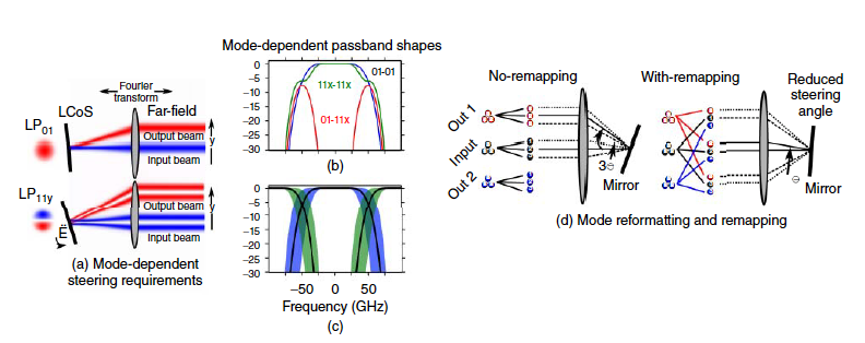
required steering angle of the switching element. Minimizing this angle allows for increasing the throughput (i.e., more modes) without decreasing switching capacity. Figure 21(b) shows two methods for routing the demultiplexed modes to a linear array, and their respective steering angle requirements. The first scenario (left half of Figure 21(b)) groups the beams by fiber such that the modes originating from the same fiber are close together.

The \(\text{LCoS}\) must steer a beam past three beams (i.e., the modes) to reach the next fiber. Alternatively, reshuffling the demultiplexed beam samples so the beams are grouped by modes (interleaved, shown in the right half of Figure 21(b)) reduces the steering angle range by a factor proportional to the number of modes. Grouping by modes places beams from different fibers close together. The \(\text{LCoS}\) only needs to steer past one beam to reach the next fiber, and all modes get routed together.

The mapping of the beam samples between the inputs and outputs are 2-2, 1-3, and 3-1. This scrambling does not degrade transmission performance, as long as the spot multiplexers have near-unitary sampling.

These spatial-diversity schemes require some more complex optics (lenses) to accommodate the increased field of view of the larger collimator array.

However, lens costs are significantly less than the cost of the steering element. With the remapping network and spatial diversity, the fiber count can be equivalent to an \(\text{SMF}\) \(\text{WSS}\) with only a marginal increase in cost. 

Figure 23 shows experimental results of an \(\text{FMF}\)-\(\text{WSS}\) built with and without spatial diversity. Figure 23(a) shows how the switch is characterized from the three \(\text{SMF}\) inputs to three \(\text{SMF}\) outputs with the spot-multiplexers used to enter and exit the \(\text{FMF}\).

We use the \(\text{SWI}\) with spatial diversity to measure the \(6\times6\) transfer matrix versus frequency between the six spatial and polarization inputs and outputs (Section Swept Wavelength Interferometry for Fibers with Multiple Spatial Paths). From the transfer matrix we obtain and plot the minimum and maximum transmission, similarly to the plots in Figure 21(b). 

Figure 23(b) shows a measurement of the output of port 1 showing flat transmission with flexible bandwidth and mode-independent passbands across the entire \(\text{C}\)-Band. Figure 23(c) and (d) compares the minimum and maximum spectral

 

 

 

 

 

transmission with and without spatial diversity for a 50-\(\text{GHz}\) interleaver between \(\text{WSS}\) outputs 1 and 2. At the passband peaks, the \(\text{WSS}\) without spatial diversity has larger \(\text{MDL}\) of 4.5 dB compared with spatial diversity 3.5 dB. Note, the \(\text{MDL}\) for the \(\text{WSS}\) with spatial diversity is consistent with four passes through the spot-multiplexers.

Its insertion loss is around 14 dB, which is also consistent with two passes through the \(\text{3D}\) waveguide (4–6 dB loss each pass), and 6-dB for losses within the switch optics (e.g., 3 dB from the \(\text{LCoS}\), and 1 dB from the grating). The losses of the 3D waveguides are not representative for the technology.

Typical loss in \(\text{3D}\) waveguide can be as small as 1 dB when coupling from \(\text{SMF}\) to \(\text{SMF}\). As expected, spatial diversity reduces the mode dependency, and can also be added with a simple design modification of the \(\text{WSS}\). 

 

SDM Fiber Amplifiers

\(\text{SDM}\) amplifiers that directly support \(\text{SDM}\) fibers potentially offer cost and complexity savings through pump and component sharing. Component sharing and pump sharing is enabled by the closely spaced or even overlapping spatial channels.

Some examples of erbium-doped fiber amplifiers \(\text{(EDFA)}\), in order of increasing integration (spatial density), are separate fibers bundled with a common coating material, multiple amplifying cores in one fiber pumped by separate pumps and by a cladding pump, and \(\text{MMF}\) amplifiers.

Long transmission fibers (10 km or more) can themselves provide gain through Raman amplification. Providing equal gain to all modes is challenging and requires optimization of the pump spatial mode, doping spatial profile, and possible external gain flattening and/or equalization. 

Figure 24 shows the differences between core pumping and cladding pumping for multicore and multimode fibers. In core-pumped amplifiers, the pump light is confined to the cores, often in the fundamental mode.

In \(\text{FMF}\) core-pumped amplifiers, exciting higher-order pump modes can reduce mode-dependent gain. Some \(\text{FMF}\) amplifiers even use more than one pump in multiple modes to further reduce the mode-dependent gain.

Cladding-pumped amplifiers distribute the pump light in the fiber cladding, which is shared by all cores and modes of the \(\text{MCFs}\). A low-index polymer coating surrounds the amplifying fiber to allow the cladding to act as a large multimode waveguide. Low-index polymers are used rather than a low-index glasses because of their much lower refractive index.

Light is launched into hundreds to thousands of cladding modes, which uniformly illuminate the entire cladding. It is then possible to use multimode pump diodes, which are generally low cost, uncooled, and have \(>10\text{W}\) output power, to illuminate the entire fiber.

The multimode pumps can be coupled into the cladding without a wavelength combiner or disturbing the cores through side pumping, v-groove coupling, or free space.

Figure 25 shows a complete amplifier that includes \(\text{(i)}\) pump combiner, \(\text{(ii)}\) amplifying fiber, \(\text{(iii)}\) isolator, and \(\text{(iv)}\) gain flattening filter. The pump combiner brings the pump and signal into the same fiber.

Common pump wavelengths are 980 and 1480 nm. In core-pumped amplifiers, the pump light is in the same

 

 

 

spatial mode/modes as the signal and a wavelength combiner is necessary to avoid passive splitting/combining loss. Even though a wavelength combiner is required, component sharing can eliminate many components that would be duplicated in parallel single-mode amplifiers.

For instance, the 19-core amplifier uses a single dichroic mirror to combine 19 pump lasers into the \(\text{MCF}\) and a single isolator to provide isolation to the 19 cores. Note, when building free-space components with more than one spatial mode/channel, it is important to use \(4f\) imaging systems to ensure equal coupling of all modes. Cladding pump amplifiers use a different set of modes (i.e., cladding modes) to guide the pump.

This eliminates the wavelength combiner through techniques such as side pumping. In side pumping, an MMF that contains the multimode pump light is tapered and brought into contact with the amplifying fiber’s cladding. The pump light can couple into the cladding with losses below 1 dB. 

A challenge in cladding-pumped amplifiers is to strongly invert the gain. An amplifier has a threshold pump intensity, \(I_{P0}\), to reach transparency. In core-pumped amplifiers, the pump intensity can be increased by using smaller cores.

The cladding area is about 100 times greater than the area of a single core, which means that the pump power of a cladding-pumped amplifier should be at least 100 times greater than that of a core-pumped amplifier to obtain equivalent performance.

The signal intensity in the core can quickly become larger than the pump intensity, especially if the cores are very small (the case for core-pumped amplifiers). When

 

 

 

the signal intensity is nearly equal to the pump intensity, the inversion decreases. The lower inversion reduces the gain, requires longer amplifying fibers, which pushes the gain toward the \(\text{L}\)-band.

However, these challenges should be solvable by decreasing the cladding area to increase the pump intensity, and increasing the size of the cores to reduce the signal intensity.

The simplicity of cladding-pumped amplifiers enables to scale the number of spatial channels without significantly increasing the amplifier cost or complexity. The main drawback of cladding-pumped amplifiers is the lack of control of the gain in individual cores. 

A per-core and spectral gain equalizer that is placed between two stages of a cladding-pumped amplifier. The gain equalizer is implemented in a free-space section and shares numerous optical components between all cores, such as the diffraction grating, the optical isolator, and a \(\text{LCoS}\) phased-array element used for attenuation.

The scheme relies on the spatial modes being separated such that they can be demultiplexed onto different positions on the \(\text{LCoS}\) attenuating array.

Gain equalization between all modes/spatial channels must be considered for all types of \(\text{SDM}\) amplifiers. In amplifiers with well-separated modes, such as multicore amplifiers, the gain can be controlled through controlling the pump power in each core, or using an external equalizer as described above.

If the cores are very uniform, multicore amplifiers should produce similar gain for all cores without additional efforts. For amplifiers with spatial overlapping channels (i.e., \(\text{FMF)}\), external equalization is more difficult. Attempting to attenuate one particular mode without affecting the others modes is difficult without using a mode multiplexer.

Therefore, it is necessary to reduce the gain variations inside the amplifier. Notable gain equalization schemes include ring doping, pump modal control, and microstructuring the gain region.

The \(\text{LP}_{01}\) mode tends to get amplified the most, whereas the higher-order modes, whose fields extend further into the cladding, see less gain medium and are amplified the least. Ring-shaped doping profiles reduce the gain for the \(\text{LP}_{01}\) mode, while enhancing the gain of the \(\text{LP}_{11}\) modes.

Higher-order modes tend to be ringlike, and launching into these modes can also enhance the gain for the higher-order modes while reducing the gain for the \(\text{LP}_{01}\) mode.

The wavelength dependence of the gain is occasionally uniform for all modes, such that wavelength equalization can be applied to all modes independently of gain equalization.

 

 

8.  CONCLUSION

\(\text{SDM}\) is the response to the limited optical transmission capacity of the \(\text{SMF}\). Multiple technological options, including multiple \(\text{SMFs}\), \(\text{MCFs}\), and \(\text{MMFs}\) and the related components such as mode couplers or fan-in/fan-out devices are now available to solve the capacity problem.

Cost reduction is expected to come mostly from integration, and in \(\text{SDM}\) systems integration will happen at various levels: the transponders, the fibers, the optical switches, and amplifiers. 

Two possible paths for \(\text{SDM}\) are conceivable: \(\text{(i)}\) systems with low crosstalk between the spatial paths and \(\text{(ii)}\) systems with \(\text{MIMO}\) \(\text{DSP}\) for crosstalk mitigation.

The second path requires more \(\text{DSP}\), but can provide higher level of component integration and, therefore, lower the component cost.

Independently from the two paths, optical switches and optical amplifiers that support multiple spatial channels are going to play a key role in \(\text{SDM}\) systems.

For optical switches, which are the key components defining optical meshed networks, the concept of “joint switching” will be essential to scale the switching capacity to the required levels.