We have considered input signals with constant power. Optical signals in any lightwave systems are in the form of a pseudo-random bit stream consisting of 0 and 1 bits. This tutorial focuses on such a realistic situation and evaluates the effects of amplifier noise on the BER and the receiver sensitivity.
1. Bit-Error Rate (BER)
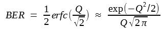
The calculation of BER for lightwave systems employing optical amplifiers follows the approach outlined in this tutorial - Optical Receiver Sensitivity. More specifically, BER is given by
However, the conditional probabilities P(0|1) and P(1|0) require knowledge of the probability density function (PDF) for the current I corresponding to symbols 0 and 1. Strictly speaking, the PDF does not remain Gaussian when optical amplifiers are used, and one should employ a more complicated form of the PDF for calculating the BER. However, the results are much simpler if the actual PDF is approximated by a Gaussian. We assume this to be the case in this tutorial.
With the Gaussian approximation for the receiver noise, we can use the analysis of the optical receiver sensitivity tutorial to find that the BER is given by the equation above, and the Q factor can still be defined as

However, the noise currents σ1 and σ0 should now include the beating terms introduced in this tutorial and are obtained using

In the case of 0 bits, σ2s and σ2sig - sp can be neglected as these two noise contributions are signal-dependent and nearly vanish for 0 bits if we assume a high extinction ratio for the bit stream. As the Q factor specifies the BER completely, one can realize a BER below 10-9 by ensuring that Q exceeds 6. The value of Q should exceed 7 if the BER needs to be below 10-12.
Several other approximations can be made while calculating the Q factor. σ2s can be neglected in comparison with σ2sig - sp in most cases of practical interest. The thermal noise σ2T can also be neglected in comparison with the dominant beating term whenever the average optical power at the receiver is relatively large (>0.1 mW). The noise currents σ1 and σ0 are then well approximated by

An important question is how receiver sensitivity is affected by optical amplification. Since the thermal noise does not appear in the equation above, one would expect that receiver performance would not be limited by it, and one may need much fewer photons per bit compared with thousands of photons required when thermal noise dominates. This is indeed the case, as also observed during the 1990s in several experiments that required about 100 to 150 photons/bit. On the other hand, as discussed in this tutorial, only 10 photons/bit are needed, on average, in the quantum limit. Even though we do not expect this level of performance when optical amplifiers are used because of the additional noise introduced by them, it is useful to inquire about the minimum number of photons in this case.
To calculate the receiver sensitivity, we assume for simplicity that no energy is contained in 0 bits so that I0 ≈ 0. Clearly,  , where
  is the average power incident on the receiver. We obtain

The receiver sensitivity can be written in terms of the average number of photons/bit,  , by using the relation
  . If we accept Δf = B/2 as a typical value of the receiver bandwidth, is given by

where rf = Δνo/Δf is the factor by which the optical filter bandwidth exceeds the receiver bandwidth.
This equation is a remarkably simple expression for the receiver sensitivity. It shows clearly why amplifiers with a small noise figure must be used. It also shows how narrowband optical filters can improve the receiver sensitivity by reducing rf. The figure below shows  as a function of rf for several values of the noise figure Fo using Q = 6, a value required to maintain a BER of 10-9. The minimum value of Fo is 2 for an ideal amplifier. The minimum value of rf is also 2 since Δνo should be wide enough to pass a signal at the bit rate B. Using Q = 6 with Fo = 2 and rf = 2, the best receiver sensitivity from the equation above is = 43.3 photons/bit. This value should be compared with = 10, the value obtained for an ideal receiver operating in the quantum-noise limit.

Even though the ASE itself has a Gaussian PDF, the detector current generated at the receiver does not follow Gaussian statistics because of the contribution of ASE-ASE beating. It is possible to calculate the probability density function of the 0 and 1 bits in terms of the modified Bessel function, and experimental measurements agree with the theoretical predictions. However, the Gaussian approximation is often used in practice for calculating the receiver sensitivity.
2. Relation between Q Factor and Optical SNR
The Q factor appearing in the calculation of BER and the optical SNR calculated in this tutorial are related to each other. To show this relationship in a simple form, we consider a lightwave system dominated by amplifier noise and assume that 0 bits carry no energy (except ASE). Then I0 ≈ 0 and I1 = RdP1, where P1 is the peak power level during each 1 bit. Using the definition of total ASE power together with

we then obtain

where we assumed M = Δνo/Δf ≫ 1.
Using the two variances from the equation above in this equation here:

we can obtain σ1 and σ0. If we calculate Q with the help of

the result is found to be:

where SNRo ≡ P1/PASE is the optical SNR. This relation can be easily inverted to find

These equations show that Q = 6 can be realized for relatively low values of optical SNR. For example, we only need SNRo = 7.5 when M = 16 to maintain Q = 6. The figure below shows how optical SNR varies with M for values of Q in the range of 4 to 8. As seen here, the required optical SNR increases rapidly as M is reduce to below 10.
